
Forces and Moments: Distributed loads
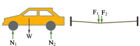
In reality, any force applied on a body is distributed over an area, i.e. a distributed load or pressure. A distributed load can be simplified (or modeled) as a concentrated force when the area of contact is relatively small and the simplification does not affect the external effects (e.g. deformation). In this case, the load on a body is referred to as a concentrated load. For example, the ground reaction forces on the tires of a car can be considered as concentrated loads to forces (Fig. 3.32). Another example is the load of a person walking on a tightrope (Fig. 3.32). If we consider the rope as a body, the person’s weight exerted to the rope through the soles of the person’s feet is the load on the rope. The forces on the rope can be regarded as concentrated forces as the contact area between the sole of each foot and the rope is small.
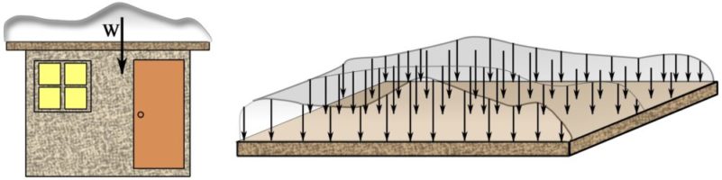
In many cases, however, a continuous distribution of forces on a body should be considered. A continuously distributed external force is referred to as a distributed load. For example, the weight of a pile of snow on a roof is distributed over the area of the roof (Fig. 3.33). This means every unit of area bears some part of the total weight of the snow pile on the roof.
A distributed load over an area has a direction and a magnitude. The direction of a distributed load over an area may vary at different points and is demonstrated by little arrows over the area. The magnitude of a distributed load is described by its intensity being defined as force per unit area, or pressure. In SI units, a distributed load has the unit of Newton per square meter  identified as Pascal,
  .
.
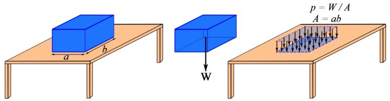
As an example, consider a solid box resting on part of the surface of a table (Fig. 3.34). The weight of the box, transmitted to the table through the base of the box that is in contact with the table, is a distributed load on the table. This load is uniformly distributed on the table as shown in Fig. 3.34. The intensity of the load is  , where
  is the weight of the box and
  is the area of the base in contact with the table. Note that,
  .
.
Uniform intensity. A distributed load with a constant intensity over an area is said to have a uniform intensity. Accordingly, a uniform load or a uniformly distributed load conveys the same meaning.
With an analogy to the weight load of a box on a surface, the magnitude of total (resultant) force exerted by a uniform load over an area is  .
.
Context: Distributed loads
- Though many loads can be idealized as a force acting at a single point there are many situations where engineers use distributed loads in design.
- Distributed loads may either be a pressure (e.g. pounds per square inch, kilopascals) or a ‘line load’ (e.g. kilonewtons per metre). Pressure loads are usually used to design wide elements like slabs and walls while line loads are used to design narrow elements like beams.
- Engineers use distributed loads to account for the self weight of elements (e.g. beams, slabs, windows, retaining walls), environmental loads (e.g. wind and snow), and internal pressures (e.g. pressurized cylinders) in structures.
- Engineers also use distributed loads to design structures where the exact arrangement of forces are unknown. For instance, engineers cannot predict how people arrange furniture and how heavy their furniture is but using historical data on living arrangements they can assume that the day-to-day pressure from people and furniture in residential buildings is 1.9 kPa (~40 pounds per square foot) when they design those types of structures.
Applications: What are situations where engineers consider distributed loads?
So far in this text we have focused on concentrated forces (or ‘point forces’). In reality, no force truly acts at a single point (discussed in Section 3.1) but assuming forces act at a single point is fine for many situations that engineers consider.
That said, there are many situations where engineers need to consider distributed loads. For instance, to ensure that the roof of the building in Fig. 3.35a does not collapse under the weight of snow, engineers need to factor in the expected depth and density of the snow on the roof as a pressure. They can determine the worst-case snow depth based on decades of climate data that is published by the federal government for each town in Canada. The same concerns (albeit harder to see) arise with wind, which can push or pull on objects.
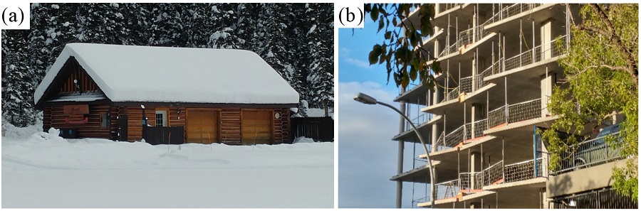
Another source of distributed loads is the actual weight of the structure itself. Reinforced concrete residential building floors (Fig. 3.35b) are typically around 200 mm thick, which translates into a pressure of around 4.5 to 5.0 kilopascals (kN/m2) which is more than double the expected loads that apartment residents (and their stuff) would have.
EXAMPLE 3.5.1
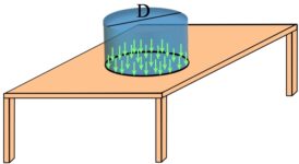
A cylinder is resting on a table an its base has a diameter of  . The weight of the cylinder is transformed to the surface of the table through the base of the cylinder and creates a uniformly distributed load with the intensity of
  . Calculate the weight of the cylinder.
SOLUTION

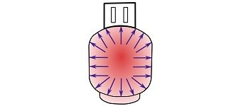
A distributed load is not necessarily distributed over a flat surface. For example, the pressure load inside a pressurized cylinder is (uniformly) distributed over the internal surface of the cylinder (Fig 3.36).
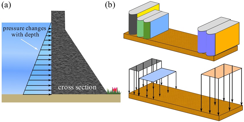
Generally, the intensity of a load varies over the area of distribution. For example, the water pressure (intensity of water load) over a dam changes with water depth (Fig. 3.37a), or the distribution of the weights of books on a shelf can have a varying intensity over the shelf (Fig. 3.37b).
Mathematically, the intensity of a load is a function of position,  , over an area. Therefore, the intensity can be defined by a function
  over the points of an area. This function can be plotted in three dimensions by considering the points of the distributed area to be on the x and y axes, and the values of intensity be along the z axis.
In this book, a special type of distributed load known as distributed load along a line or an axis is considered. Realistic loads in many problems in engineering practice are modeled or closely represented by this type of loading.
Distributed load along an axis
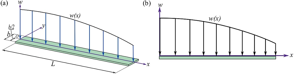
A distributed load over an area may only vary along one direction or axis and be constant in another direction. Consider a distributed load over the top surface of a rectangular plate as shown in Fig. 3.38. A Cartesian coordinate system is placed on the plate with its origin,  , located at one end of the plate, and the x axis along the center line of the width of the plate (the y axis is parallel to the width of the plate). The intensity of the load, is a function of x and y over the area of the plate.
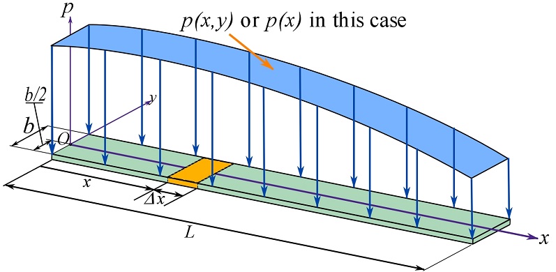
In this case, the intensity of the load,  is constant along the y axis. Therefore, the intensity only depends on x and can be described by a function of x as
  . It is more convenient to define an intensity function that describes the load per unit length instead of per unit area by writing
  . The unit of
  in the SI system is Newton per meter,
  . The load described by is applied along the x axis (Fig. 3.39a). A two dimensional representation of Fig. 3.39a as shown in Fig. 3.39b is sufficient for most analyses.
In many engineering problems, we need to find the approximate value of . One example is given here to clarify the concept of load per unit length.
EXAMPLE 3.5.2
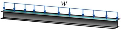
The photo Lunch atop a Skyscraper (1932), shows eleven ironworkers sitting on a beam. If the average mass of each man is assumed  , determine their weight load distributed over the length (axis) of the beam. Assume that the length of the beam over which the men are sitting is
  .
.

SOLUTION
The total weight to be distributed along the axis of the beam is  . Therefore,

which is constant over the length as shown in the figure below.
Simplification of a distributed load along an axis
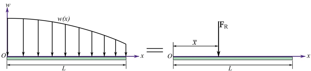
In many problems, like equilibrium of rigid bodies (Section 5.2) or support reaction calculation a distributed load can be represented by a concentrated load, for simplicity reasons, without changing its effects in the calculation. The equivalent system of a distributed load as shown in Fig. 3.40 consists of a resultant force at a specific location. The equivalent system is obtained based on the simplification of a coplanar force system to a resultant force (see Section 3.4.2 and example 3.4.5).
In many problems the shape of the load intensity function is simple and  can be readily calculated. Figure 3.41 shows the resultant force and of two common load distributions.
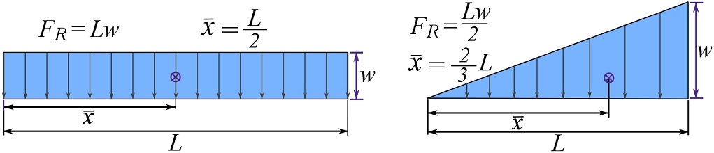
The magnitude of the resultant force is the area under the intensity function and is the  coordinate of the centroid of the shape of the area under the intensity function. The following paragraphs show the general calculation of
  and . Students are encouraged to read them after acquiring a firm knowledge in calculus.
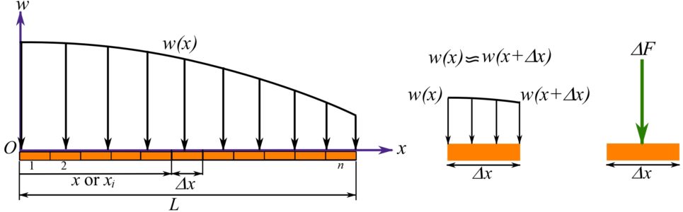
To determine the magnitude of the resultant force, the total length  of the distributed load is divided into
  equal-length elements (segments) with a length of
  (Fig. 3.42). If
  is small enough, is almost uniform over the element and, therefore, the magnitude of the force over the element is
  . The magnitude of is approximately determined by summing
  over as,
![\[F_R\approx +\downarrow\sum_{i=1}^{n}\Delta F_i=\sum_{i=1}^{n}w(x_i)\Delta x\]](https://engcourses-uofa.ca/wp-content/ql-cache/quicklatex.com-9614010016a0cdd0c217dcacdada400f_l3.png "Rendered by QuickLaTeX.com")
The exact value of is obtained by letting the number of divisions, , increase to infinity,
![\[F_R=\lim_{n\to \infty}\sum_{i=1}^{n}\Delta F_i=\lim_{n\to \infty}\sum_{i=1}^{n}w(x_i)\Delta x\]](https://engcourses-uofa.ca/wp-content/ql-cache/quicklatex.com-52b9e1523bac33d0c73402b547327b1d_l3.png "Rendered by QuickLaTeX.com")
leading to,
(3.27) ![\[F_R =\int_0^Lw(x)dx \]](https://engcourses-uofa.ca/wp-content/ql-cache/quicklatex.com-3814dd01a3bccc1555abfa626668c28b_l3.png "Rendered by QuickLaTeX.com")
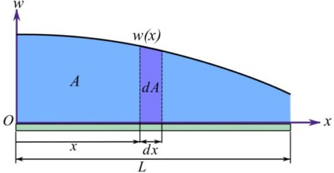
The geometrical interpretation of this integral is the area, , under the load intensity function ,
(3.28) ![\[F_R=A=\int_0^Lw(x)dx=\int_A dA \]](https://engcourses-uofa.ca/wp-content/ql-cache/quicklatex.com-414fe34f4ede1756fd73583797d0acdd_l3.png "Rendered by QuickLaTeX.com")
where  is an element of area as shown in Fig. 3.43.
The location of  is determined by equating the moments of the forces about a point in the two systems (Fig. 3.40). The point for calculating the moments can be anywhere on the x axis, however, it is common to select any end of the length over which the load is distributed. We select point located at the origin of the x axis (Fig. 3.40). Equating the moments of the two systems is written as,
![\[\underset{\text{System 1}}{(\bold M_R)_O}=\underset{\text{System 2}}{(\bold M_R)_O}\implies\bar xF_R=\lim_{n\to \infty}\sum_{i=1}^{n}x_i\Delta F_i=\lim_{n\to \infty}\sum_{i=1}^{n}x_iw(x_i)\Delta x\]](https://engcourses-uofa.ca/wp-content/ql-cache/quicklatex.com-30632e43c4e1dc53f90e9a5e7c67eb2c_l3.png "Rendered by QuickLaTeX.com")
which becomes equivalent to the following integral,
![\[\bar x F_R=\int_0^Lxw(x)dx\]](https://engcourses-uofa.ca/wp-content/ql-cache/quicklatex.com-543200a3818e6379bf15a92512d1cce3_l3.png "Rendered by QuickLaTeX.com")
and (by Eq. 3.27) leads to,
(3.29) ![\[\bar x=\frac{\int_0^Lxw(x)dx}{\int_0^Lw(x)dx} \]](https://engcourses-uofa.ca/wp-content/ql-cache/quicklatex.com-c0373ab2f46a36a0e179d1236c8bc0e9_l3.png "Rendered by QuickLaTeX.com")
Considering the geometrical meaning of this integration (Fig. 3.43), we write Eq. 3.29 as,
(3.30) ![\[\bar x=\frac{\int_AxdA}{A} \]](https://engcourses-uofa.ca/wp-content/ql-cache/quicklatex.com-44f3699457b703517b53fe738a33391f_l3.png "Rendered by QuickLaTeX.com")
which can be regarded as the geometrical interpretation of Eq. 3.29. The point associated with the coordinate is a geometrical properties of the shape of the area under the diagram (graph) of the load intensity function. This is called the coordinate of the centroid of the shape of the area. The concept of centroid will be presented in Section 9.3.