
Internal Forces: Relationships between Load, Shear, and Moments
Direct derivation of the functions  and
and  by the method of sections may be tedious. The direct application of the method of sections can be avoided by deriving the relationship between the load, shear, and bending moment. In this section, four relationships are derived:
1- point force AND shear
2- distributed load AND shear
3- shear AND bending moment
4- couple moment AND bending moment
1- Point Force and Shear
Consider a downward point force acting at a point  of a beam (Fig. 7.16a). To find the relationship between the shear and the point force, a segment of the beam as shown in Fig. 7.16a is considered. The segment contains the force (point of application) and has a fractional length of
  .
.
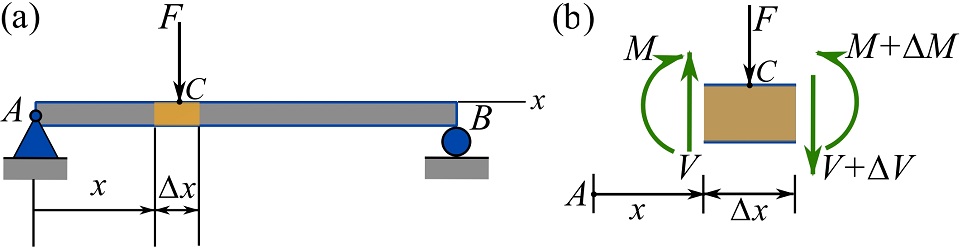
Isolating the segment exposes the internal forces on its FBD as shown in Fig. 7.16b. The beam is free of axial load. The values of the function and , evaluated at  , are denoted as
  and
and  respectively. At a distance
  away from point , the shear force and the bending moment generally vary to
  and
and  . The force equilibrium for the free segment is,
![\[+\uparrow \sum F_y = 0\implies V-F-(V+\Delta V)=0\implies \Delta V=-F\]](https://engcourses-uofa.ca/wp-content/ql-cache/quicklatex.com-12b31efd0f8efdc7b0ef5da2e62084bc_l3.png "Rendered by QuickLaTeX.com")
which can be written as,
(7.1) ![\[\Delta V = -F\quad \text{or}\quad V_{C^+}-V_{C^-}=-F\]](https://engcourses-uofa.ca/wp-content/ql-cache/quicklatex.com-40cf2ad6b10a560b65aab8687c99332e_l3.png "Rendered by QuickLaTeX.com")
where  and
and  denote the shear right before and after point respectively.
Equation 7.1 states that a point force  acting on a beam creates a jump, with a magnitude of
  , in the values of . The jump appears as a jump discontinuity in the diagram of .
Remark: exactly at the application point of a point force, the value of shear is undefined due to the jump discontinuity.
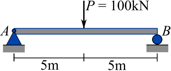
EXAMPLE 7.3.1
Plot the shear diagram of the beam shown. Use Eq. 7.1.
SOLUTION
Draw the FBD of the beam and solve for the support reactions.
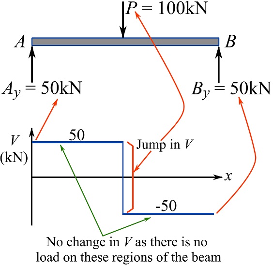
The FBD with solved support reactions are demonstrated in the figure below.
Start from the known shear at point  and use
  to determine the shear along the beam axis. Observe the jump in the values of at the point where the external load
  acts; the jump in values is
  .
.
2- Distributed load and Shear
Consider a beam under a continuous distributed load expressed by a function  . As shown in Fig. 7.17a, positive values of are associated with downward force on the beam.
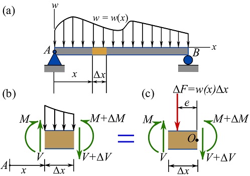
To obtain the relationship between and , a beam segment with a fractional length is considered at an arbitrary distance from the left-hand side of the beam (Fig. 7.17a). The FBD of the segment is constructed as shown in Fig 7.17b. The beam is free of axial load. The shear force and the bending moment at are denoted as and respectively. The shear force and bending moment at a distance are denoted as and respectively.
As shown in Fig 7.17c, the part of the distributed load, , acting on the segment is replaced with its (equivalent) resultant force with the magnitude of  . The location at which
  acts on the segment is shown by
  in the figure. In fact, acts somewhere along the length of the segment; in other words,
  where
where  . It will be seen that the location of does not affect the calculations. Writing the force equation of equilibrium for the FBD of the segment leads to the following relationship.
![\[+\uparrow \sum F_y = 0\implies V-\Delta F-(V+\Delta V)=0\implies \frac{\Delta V}{\Delta x}=-w(x)\]](https://engcourses-uofa.ca/wp-content/ql-cache/quicklatex.com-ff0322e10b897acb02b28f1b33d2154a_l3.png "Rendered by QuickLaTeX.com")
Therefore, letting  and taking the limit of both sides as,
![\[\lim_{\Delta x \to 0} \frac{\Delta V}{\Delta x}=-w(x)\]](https://engcourses-uofa.ca/wp-content/ql-cache/quicklatex.com-29c001584f86c161cd31bdb098dce7ff_l3.png "Rendered by QuickLaTeX.com")
leads to,
(7.2) ![\[\frac{dV}{dx}=-w(x)\]](https://engcourses-uofa.ca/wp-content/ql-cache/quicklatex.com-1c4cc0ab11e8b7dd6ef746ac17506e85_l3.png "Rendered by QuickLaTeX.com")
This equation indicates that at any point along the axis of the beam, the slope of the diagram of equals the negative value of . This is the geometrical interpretation of Eq. 7.2.
An alternative form of the relationship between and is obtained by writing Eq. 7.2 as  and integrating both sides,
![\[\int_a^bdV=\int_a^b -w(x)dx\]](https://engcourses-uofa.ca/wp-content/ql-cache/quicklatex.com-7c1e0bc0eda0f46dd8b673749e9d0760_l3.png "Rendered by QuickLaTeX.com")
leads to,
(7.3) ![\[V|_{x=b}-V|_{x=a}=\int_a^b -w(x)dx\]](https://engcourses-uofa.ca/wp-content/ql-cache/quicklatex.com-6294a169a5dee90634049620dbd873b7_l3.png "Rendered by QuickLaTeX.com")
where  and
and  such that
  are the coordinates of two points and
  on the axis of the beam.
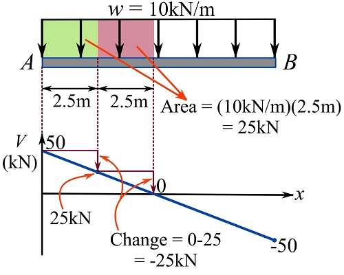
The geometrical interpretation of Eq. 7.3 indicates that the variation of the shear between two points on the beam equals the area (negative value) under the distributed load between the two points.
Equation 7.3 can be utilized to find . If the shear,  is known at a starting point,
  , then the shear at any arbitrary point with the coordinate
  is,
is,
(7.4) ![\[V(x)=V_A - \int_a^x w(t)dt\]](https://engcourses-uofa.ca/wp-content/ql-cache/quicklatex.com-cb13d6165004270f4655d37bc4b7c9b7_l3.png "Rendered by QuickLaTeX.com")
Note that the integration variable is a dummy variable and therefore renamed to  .
.
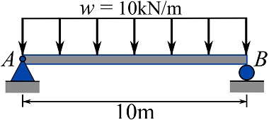
EXAMPLE 7.3.2
For the loaded beam shown.
1- Plot the shear diagram of the beam. Use Eq. 7.4.
2- Using the geometrical interpretation of the relationship between external load and shear force, show that  and
and  at
at  and
and  respectively.
SOLUTION
Part 1
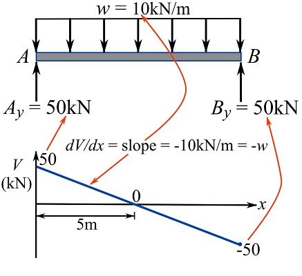
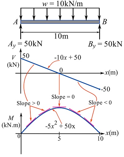
Draw the FBD of the beam and solve for the support reactions.
The FBD with solved support reactions are demonstrated in the figure below.
Starting from point , determine the shear at any point using Eq. 7.4 as,
![\[V(x)=V_A - \int_a^x w(t)dt=50-\int_0^x 10dt=50 -10x\text{ kN}\]](https://engcourses-uofa.ca/wp-content/ql-cache/quicklatex.com-d971dcd3a7c0aba482b7d28ac855ac2e_l3.png "Rendered by QuickLaTeX.com")
Observe the relationship between and the slope of ; the slope,  is constant as
  is constant.
Part 2
Use the relationship 
3– Shear and Bending Moment.
Shear and moment relationship can be obtained by writing the moment equation of equilibrium about point  of the free segment shown in Fig. 7.17c as,
![\[\begin{split}\circlearrowleft{+} \sum M_O=0 &\implies -M-(V)(\Delta x) + (\Delta F)(e)+(M+\Delta M)=0\\&\implies -(V)(\Delta x)+(w(x)\Delta x)(k\Delta x)+\Delta M=0\\&\implies -(V)(\Delta x)+(kw(x))(\Delta x)^2+\Delta M=0\\&\implies V=(kw(x))(\Delta x)+\frac{\Delta M}{\Delta x}\end{split}\]](https://engcourses-uofa.ca/wp-content/ql-cache/quicklatex.com-f11714867c0590147f09e1025ef873dc_l3.png "Rendered by QuickLaTeX.com")
and letting ,
(7.5) ![\[V=\frac{dM}{dx} \]](https://engcourses-uofa.ca/wp-content/ql-cache/quicklatex.com-2908ee86965735eaa80e974a69946f13_l3.png "Rendered by QuickLaTeX.com")
This relationship indicates that at any point along the axis of the beam, the slope of the diagram of equals the value of .
The integral form of Eq. 7.5 is achieved by writing  and integrating both sides as,
(7.6) ![\[M|_{x=b}-M|_{x=a}=\int_a^b V(x)dx\]](https://engcourses-uofa.ca/wp-content/ql-cache/quicklatex.com-1b06a62918299e5bfb9939d4a5931f8a_l3.png "Rendered by QuickLaTeX.com")
Equation 7.6 indicates that the variation of the bending moment between two points on the beam equals the area under the shear diagram between the two points.
Using Eq. 7.6, the function can be determined. If the bending moment,  is known at a starting point, , then the bending moment at any arbitrary point with the coordinate is,
(7.7) ![\[M(x)=M_A + \int_a^x V(t)dt\]](https://engcourses-uofa.ca/wp-content/ql-cache/quicklatex.com-df2e4e0e06c355694970dfd4c457589a_l3.png "Rendered by QuickLaTeX.com")
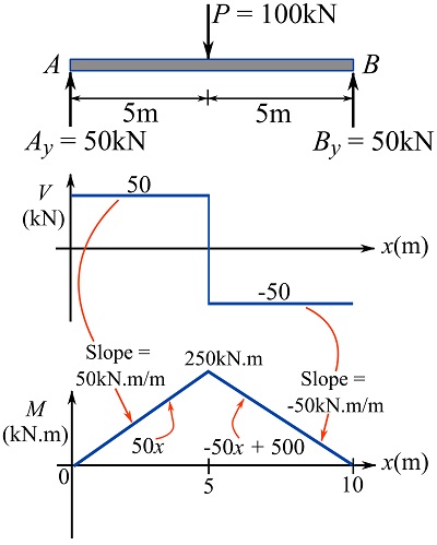
EXAMPLE 7.3.3
For the loaded beam shown.
1- Plot the moment diagram of the beam. Use Eq. 7.7.
2- Using the geometrical interpretation of the relationship between shear and bending moment, show that  at .
at .
SOLUTION
Part 1
Drawing the FBD, obtaining the support reactions, and drawing the shear diagram are already done and demonstrated in Example 7.3.1.
To determine , use Eq. 7.7 for  and
and  .
.
For ,
![\[\begin{split}M(x)&=M_A + \int_0^x V(t)dt=0+\int_0^x 50dt\\&\therefore M(x)=50x\text{ kN.m}\quad 0\le x\le 5\end{split}\]](https://engcourses-uofa.ca/wp-content/ql-cache/quicklatex.com-adc3b0f6f10265e86a27bab2ee07586c_l3.png "Rendered by QuickLaTeX.com")
For ,
![\[\begin{split}M(x)&=M_A + \int_0^x V(t)dt=0+\int_0^5 50dt+\int_5^x -50dt\\&\therefore M(x)=500 -50x \text{ kN.m}\quad 5\le x\le 10\end{split}\]](https://engcourses-uofa.ca/wp-content/ql-cache/quicklatex.com-e1b4769409e0ec297e3c00486be3d6ec_l3.png "Rendered by QuickLaTeX.com")
Therefore,
![\[M(x)=\begin{cases}50x\text{ kN.m}\quad 0\le x\le 5\\-50x+500 \text{ kN.m}\quad 5\le x\le 10\end{cases}\]](https://engcourses-uofa.ca/wp-content/ql-cache/quicklatex.com-456ac52e330412302096dad555d66adf_l3.png "Rendered by QuickLaTeX.com")
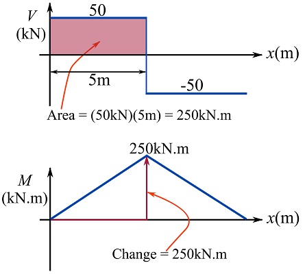
The diagram of is as follows,
Part 2
Use the relationship  .
.
![\[\begin{split}\Delta M &= M(5)-M(0)=(50\text{kN.m})(5\text{m})=250\text{ kN.m}\\&\therefore M(5)= 250\text{ kN.m}\end{split}\]](https://engcourses-uofa.ca/wp-content/ql-cache/quicklatex.com-a007d8dc1cc2378e59403f0b0521fa9a_l3.png "Rendered by QuickLaTeX.com")
EXAMPLE 7.3.4
For the loaded beam shown.
1- Plot the moment diagram of the beam. Use Eq. 7.7.
2- Using the geometrical interpretation of the relationship between shear and bending moment, show that  at .
at .
3- Show that the change  equals the area under diagram.
SOLUTION
Part 1
Drawing the FBD, obtaining the support reactions, and drawing the shear diagram are already done and demonstrated in Example 7.3.2.
To determine , use Eq. 7.7 for  .
.
![\[\begin{split}M(x)&=M_A + \int_0^x V(t)dt=0+\int_0^x -10x+50dt\\&\therefore M(x)=-5x^2+50x\text{ kN.m}\end{split}\]](https://engcourses-uofa.ca/wp-content/ql-cache/quicklatex.com-f4d1ef62c8f7e9aec27eb8a223bba335_l3.png "Rendered by QuickLaTeX.com")
The diagram of is as follows,
Part 2
Use the relationship .
![\[\begin{split}\Delta M&=M(5)-M(0)=(50\text{kN})(5m)/2=125\text{ kN.m}\\&\therefore M(5)= 125\text{ kN.m}\end{split}\]](https://engcourses-uofa.ca/wp-content/ql-cache/quicklatex.com-8c28ab008f808a500c089dadbfa7d2d5_l3.png "Rendered by QuickLaTeX.com")
See figure below for the demonstration.
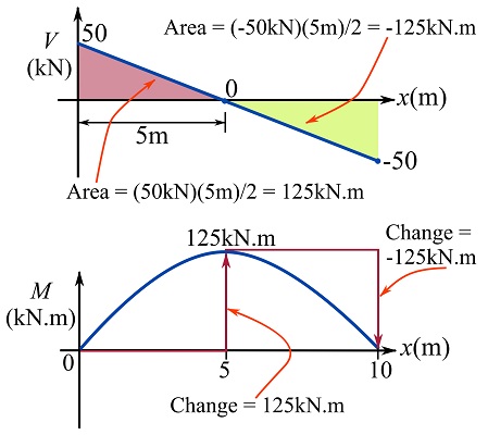
Part 3
![\[\begin{split}\Delta M&=M(10)-M(5)=(50\text{kN})(5m)/2=125\text{ kN.m}\&\implies 0 - 125= -125\text{ kN.m}\\&\therefore -125=-125\end{split}\]](https://engcourses-uofa.ca/wp-content/ql-cache/quicklatex.com-dde1532b3b6561112af62247a548fe19_l3.png "Rendered by QuickLaTeX.com")
See the above figure for the demonstration.
4- Couple Moment and Bending Moment
Consider an external couple moment acting at a point of a beam (Fig. 7.18a). To find the relationship between the bending moment and the couple moment, a segment of the beam as shown in Fig. 7.18a is considered.
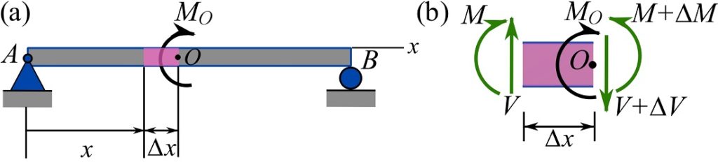
The FBD of the segment is shown in Fig 7.18b. Writing the moment equation of equilibrium for the free segments lead to,
![\[\circlearrowleft{+} \sum (M)_O=0 \implies -M-M_O-(V)(\Delta x) +(M+\Delta M)=0\implies -M_O-(V)(\Delta x) + \Delta M=0\]](https://engcourses-uofa.ca/wp-content/ql-cache/quicklatex.com-ddeb4ddefa98ae72e33be3341cbee1d7_l3.png "Rendered by QuickLaTeX.com")
Letting  , results in,
(7.8) ![\[\Delta M = M_O\quad \text{or}\quad M_{O^+}-M_{O^-}=M_O\]](https://engcourses-uofa.ca/wp-content/ql-cache/quicklatex.com-a6236f08821a3713ffc0b44b3859d7ea_l3.png "Rendered by QuickLaTeX.com")
where  and
and  denote the bending moment right before and after point respectively.
Equation 7.9 states that a couple moment  acting on a beam creates a jump, with a magnitude of , in the values of . The jump appears as a jump discontinuity in the diagram of .
Remark: the value of bending moment exactly at the application point of a couple moment is undefined due to the jump discontinuity.
Use the following interactive tool to obtain SFD and BMD of different beams (simply supported and cantilever beams) with different supports and loads. Observe the variations within each diagram upon changing the loads and other inputs.
Note that the numerical results may contain negligible error due to round off. Also, In some cases you may observe that the support reaction of the roller becomes a pulling force on the beam. In this case, assume that the support is a roller in a frictionless slot