
Equilibrium of Particles and Rigid Bodies: Equilibrium of a particle
Two- and three- dimensional force equilibrium
An object can be idealized as a particle with negligible size and with or without mass. When forces are acting on a particle, they do not create moment tendency on the particle. See Chapter 1 for further explanation of particles.
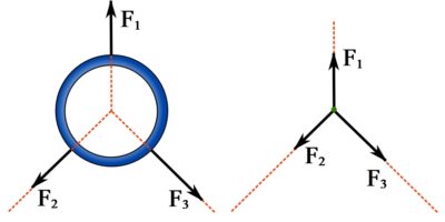
Whether a body can be considered as a particle or not depends on the problem and the information we would like to calculate for. For example, a ring shown in Fig. 5.1 is subjected to three forces with their lines of action all meeting at the center of the ring. Due to the transmissivity of the forces, the forces can slide (along their lines of action) to meet at the center without changing their effects . Therefore, the system can be treated as three forces acting at a particle located at the center of the ring.
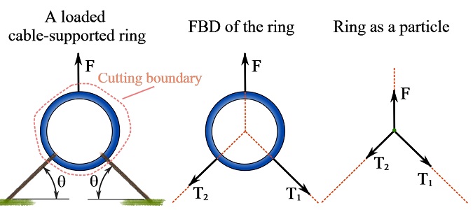
A free body diagram (FBD) can be used to facilitate the analysis of forces. The FBD of a particle is achieved by isolating the particle from its surrounding (free particle). The FBD of a particle consists of the particle, represented as a point, and concurrent forces acting on the particle. See more information on FBD in Chapter 4 . As an example, Fig. 5.2 demonstrates how a ring being pulled by three cable forces is idealized as a particle subject to three forces.
A particle is said to be in equilibrium if it was originally at rest or moving along a straight line with constant velocity, and remains so. According to Newton’s first law of motion, if a particle is in equilibrium, the resultant forces of all the force acting on it must be zero, expressed as the equation of equilibrium (of a particle),
(5.1) ![\[\bold F_R = \sum \bold F=\bold 0 \]](https://engcourses-uofa.ca/wp-content/ql-cache/quicklatex.com-c29f8a041f70761aba815ae7bc736355_l3.png "Rendered by QuickLaTeX.com")
The equation of equilibrium includes the necessary and sufficient conditions for a particle to be in equilibrium. In Statics, mainly non-moving (at-rest) bodies are considered; in other words, static equilibrium of a stationary body or structure is concerned.
The equation of equilibrium can be separately considered for coplanar and spatial force systems.
Equations of equilibrium for coplanar force systems (two dimensions)
Let  be a system of coplanar forces acting on a particle. If each force is resolved into two perpendicular components in the x and y directions of a Cartesian coordinate system, Eq. 5.1 for the particle in equilibrium is written as,
(5.2) ![\[\begin{split}\bold F_{Rx} &= \sum_i^n \bold F_{ix}=\bold 0 \\\bold F_{Ry} &=\sum_i^n \bold F_{iy}=\bold 0 \end{split}\]](https://engcourses-uofa.ca/wp-content/ql-cache/quicklatex.com-b657bc6a0321cf9fe90c386a6617d626_l3.png "Rendered by QuickLaTeX.com")
meaning that equilibrium of a particle subjected to forces is maintained if the sum of the force components in each direction is zero.
Equations 5.2 state that the magnitude of the resultant force is zero. Therefore, they can be written in terms of the magnitudes of the force components. Based on the magnitude-based notation and scalar formulation introduced in the beginning of Section 3.2, Eq. 5.2 can be written as,
(5.3) ![\[\begin{split}\rightarrow \sum F_x&=0\\\uparrow \sum F_y&=0\end{split}\]](https://engcourses-uofa.ca/wp-content/ql-cache/quicklatex.com-609870ef96c8181966980842ae69080c_l3.png "Rendered by QuickLaTeX.com")
where the sum is over all forces acting on the particle, and each  and
and  is the magnitude of a force component. The arrows
  and
and  indicate the positive direction of the x and y axes respectively. Thereby, the magnitudes of force components in the positive direction of their corresponding Cartesian axes appear with positive signs in the sum. Accordingly, the magnitudes of force components in the negative direction of their corresponding Cartesian axes appear with minus signs in the sum.
Equations 5.3 can be referred to as the scalar Cartesian equations of equilibrium.
The equations of equilibrium can be used to determine unknown internal forces or support reactions in a problem. For example, The cable forces in the case of the ring shown in Fig. 5.2 are unknown. However, if the particle (ring) is in equilibrium, the equations of equilibrium are utilized to determine the unknown forces.
EXAMPLE 5.1.1
For the ring shown, If  and
and  , determine the tension forces,
  and
and  , in the cables.
SOLUTION
Consider the ring as a particle and draw the FBD of the ring.
Find the Cartesian (rectangular) components of each force (set a Cartesian coordinate system if not given).
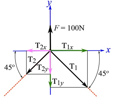
Use the scalar formulation. Determine the magnitudes of the components of the (known and unknown) forces by decomposing them into their Cartesian components.
![\[\begin{split}\bold F &=\bold F_x + \bold F_y\implies F_x=0,\quad F_y=100\text{ N}\uparrow \\\bold T_1 &=\bold T_{1x} +\bold T_{1y}\implies T_{1x}=T_1\cos 45^\circ\text {N}\rightarrow, \quad T_{1y}=T_1\sin 45^\circ\text {N}\downarrow\\\bold T_2&=\bold T_{2x}+\bold T_{2y} =\implies T_{2x}=T_2\cos 45^\circ\text{ N}\leftarrow, \quad T_{2y}=T_2\sin 45^\circ\text { N}\downarrow\end{split}\]](https://engcourses-uofa.ca/wp-content/ql-cache/quicklatex.com-902b9a7cf8727f9b829c46b68ca4ee3c_l3.png "Rendered by QuickLaTeX.com")
where the non-bold capital letters are magnitudes and hence non negative.
Apply the equilibrium equation in each direction.
![\[\begin{split}\overset{+}{\rightarrow}\ \sum F_x&=0 \implies \frac{\sqrt{2}}{2}T_1-\frac{\sqrt{2}}{2}T_2=0\implies T_1-T_2=0\\+\uparrow\ \sum F_y&=0\implies -\frac{\sqrt{2}}{2}T_1-\frac{\sqrt{2}}{2}T_2+100=0\implies T_1+T_2=100\sqrt{2}\end{split}\]](https://engcourses-uofa.ca/wp-content/ql-cache/quicklatex.com-fc131e482480352466a1c8b1651da79e_l3.png "Rendered by QuickLaTeX.com")
Solve the system of equations for the unknowns.
![\[\begin{cases}T_1 - T_2 = 0\\T_1+T_2=100\sqrt{2}\end{cases}\]](https://engcourses-uofa.ca/wp-content/ql-cache/quicklatex.com-b401e98899106a49bb8e29ce00980d57_l3.png "Rendered by QuickLaTeX.com")
Leading to,
![\[T_1=T_2=100\frac{\sqrt{2}}{2}\text { N}= 70.7\text { N}\]](https://engcourses-uofa.ca/wp-content/ql-cache/quicklatex.com-3cc8d49e2e2a42bf7d5c7e35aec431b4_l3.png "Rendered by QuickLaTeX.com")
In two-dimensional problems, there are two equations of equilibrium (Eq. 5.2) for a system of forces acting on a particle in equilibrium, indicating there can be maximum two unknowns.
In the previous example, the unknowns were the magnitudes of two internal cable forces. Note that the directions of the forces were already known by the geometrical setting (i.e. angles of the cables) and nature of the cables (can only be in tension). In other problems, directions can also be the unknowns.
If the direction of a force is unknown (in addition to its magnitude), the direction, including the sense of direction, of the force should be assumed. To this end, an (unknown) angle,  , from an axis quantifies the direction of the force. Therefore, the unknowns of the equilibrium equations are
  (the force magnitude) and . Solving a system of equations with as its unknowns may lead to a negative value for . In such a case, the sense of direction (arrowhead) of
  has to be switched.
The following examples present the approach of assuming the direction of an unknown force.
EXAMPLE 5.1.2
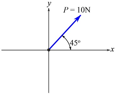
Find the force that establishes the equilibrium conditions for the particle subjected to the force shown.
SOLUTION
Since in addition to its magnitude, the direction of the force needed for the particle equilibrium is unknown, assume the direction (and its sense) of the force as measured from the positive x axis (figure below).
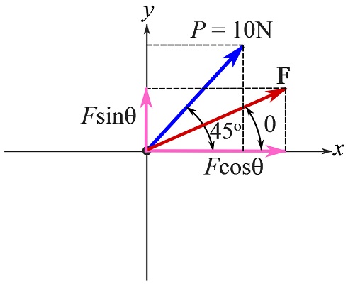
Use the scalar formulation. Determine the magnitudes of the components of the (known and unknown) forces by decomposing them into their Cartesian components.
![\[\begin{split}\bold P&=\bold P_x + \bold P_y\\&\implies P_x=10\cos 45^\circ\text { N}\rightarrow, \qquad P_y=10\sin 45^\circ\text { N} \uparrow\\\bold F&=\bold F_x + \bold F_y\\&\implies F_x=F\cos\theta\text { N}\rightarrow, \qquad F_y=F\sin\theta\text { N}\uparrow\end{split}\]](https://engcourses-uofa.ca/wp-content/ql-cache/quicklatex.com-beafa36e901c2e9cc5975d8f75237b2b_l3.png "Rendered by QuickLaTeX.com")
Write the equilibrium equations. The Cartesian axes set the positive direction for the equilibrium equations.
![\[\begin{split}\overset{+}{\rightarrow}\ \sum F_x&=0 \implies F\cos\theta-150+10\cos 45^\circ=0 \\+\uparrow\ \sum F_y&=0\implies F\sin\theta+0+10\cos 45^\circ=0\end{split}\]](https://engcourses-uofa.ca/wp-content/ql-cache/quicklatex.com-4a468cb50ea615688e4523ea7d0046c9_l3.png "Rendered by QuickLaTeX.com")
leading to the following system of equations,
![\[\begin{cases}F\cos\theta=-7.07\text { N}\\F\sin\theta=-7.07\text { N}\end{cases}\]](https://engcourses-uofa.ca/wp-content/ql-cache/quicklatex.com-b9ca841b25ff32fd02e0f33f686a004a_l3.png "Rendered by QuickLaTeX.com")
Solving the system of equations by the substitution method (substitute for ), you can write,
![\[\frac{\sin \theta}{\cos \theta}=\frac{-7.07}{-7.07}\implies \tan \theta=1.0\implies \theta=\arctan (1.0)= 45^\circ\]](https://engcourses-uofa.ca/wp-content/ql-cache/quicklatex.com-f5da51db16c9a263672de3110e1b238d_l3.png "Rendered by QuickLaTeX.com")
Note that the range of the function  is
is  . The angle determines the angle of the line of action of the force with the x axis. To find and its sense of direction, solve any of the equilibrium equations for ,
![\[\begin{split}&F\cos 45^\circ=-7.07\text { N}\\&\therefore F=-10\text{ N}\end{split}\]](https://engcourses-uofa.ca/wp-content/ql-cache/quicklatex.com-80016552074654e6c657eff4f8c6f0b8_l3.png "Rendered by QuickLaTeX.com")
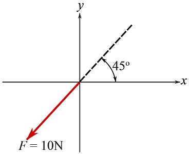
Because the magnitude of turned out to be negative, you should switch its sense of directions that previously assumed. Consequently, with its true direction is shown as,
Although the answer to this problem could have been easily found by setting the unknown force equal in magnitude but with the opposite direction to  , i.e.
  , it was intended to demonstrate a systematic way of solving the problem.
EXAMPLE 5.1.3
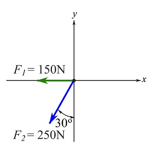
Find the force that establishes the equilibrium conditions for the particle subjected to the forces shown.
SOLUTION
Assume the direction (and its sense) of the unknown force as measured from the positive x axis (figure below).
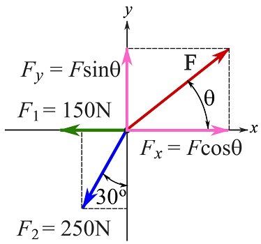
Use the scalar formulation. Determine the magnitudes of the components of the (known and unknown) forces by decomposing them into their Cartesian components.
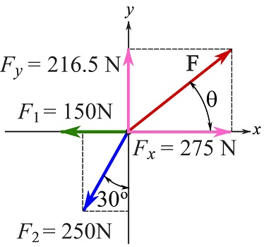
![\[\begin{split}\bold F_1&=\bold F_{1x} + \bold F_{1y}\\&\implies F_{1x}=150\text { N}\leftarrow,\qquad F_{1y}=0\text { N}\\\bold F_2&=\bold F_{2x} + \bold F_{2y}\\&\implies F_{2x}=250\sin30^\circ\text { N}\leftarrow, \qquad F_{2y}=250\cos30^\circ\text { N}\downarrow\\\bold F&=\bold F_{x} + \bold F_{y}\\&\implies F_x=F\cos\theta\text { N}\rightarrow,\qquad F_y=F\sin\theta\text { N}\uparrow\end{split}\]](https://engcourses-uofa.ca/wp-content/ql-cache/quicklatex.com-9abaee852a11837fbfba22e28af37af3_l3.png "Rendered by QuickLaTeX.com")
Write the equilibrium equations. The Cartesian axes set the positive direction for the equilibrium equations.
![\[\begin{split}\overset{+}{\rightarrow}\ \sum F_x&=0 \implies F\cos\theta-150-250\sin 30^\circ=0 \\+\uparrow\ \sum F_y&=0\implies F\sin\theta+0-250\cos 30^\circ=0\end{split}\]](https://engcourses-uofa.ca/wp-content/ql-cache/quicklatex.com-ff68a6fcf14b5fd4e4fa862a3b1ae11d_l3.png "Rendered by QuickLaTeX.com")
leading to the following system of equations,
![\[\begin{cases}F\cos\theta=150+250\sin 30^\circ=275\text { N}\\F\sin\theta=250\cos 30^\circ=216.5\text { N}\end{cases}\]](https://engcourses-uofa.ca/wp-content/ql-cache/quicklatex.com-a1783373f84839f1e500eb381d9f3407_l3.png "Rendered by QuickLaTeX.com")
Solving the system of equations by the substitution method (substitute for ), you can write,
![\[\frac{\sin \theta}{\cos \theta}=\frac{216.5}{275}\implies \tan \theta=\frac{216.5}{275}\implies \theta=\arctan (0.79)= 38.3^\circ\]](https://engcourses-uofa.ca/wp-content/ql-cache/quicklatex.com-1a0d01d824924ca043386fd53ad39302_l3.png "Rendered by QuickLaTeX.com")
Now that is determined, you can use any of the equations to determine the magnitude, of the force. For instance,
![\[\begin{split}&F\cos38.3^\circ=275\text { N}\\&\therefore F= 350\text{ N}\end{split}\]](https://engcourses-uofa.ca/wp-content/ql-cache/quicklatex.com-6dc0946df9c59e255d71dc8f1586d454_l3.png "Rendered by QuickLaTeX.com")
In the above examples, the equations directly contained the unknown magnitude of the force, , and its direction measured by . Although this method is totally valid, the calculations become simpler if the magnitudes of the components of the unknown force are directly involved. To this end, and directly enter the scalar formulations. After solving the system of equations for and , their signs indicate their senses of directions along the x and y axes. The magnitude of and its angle with any axis can then be readily obtained if needed. The following examples clarify the method.
EXAMPLE 5.1.4
Solve Example 5.1.3 again by directly involving the magnitudes of the components of the unknown force in the scalar formulation of the equations of equilibrium.
SOLUTION
Assume the direction (and its sense) of the unknown force . The direction can be arbitrary. In this example choose the direction of such that  and
and  are directed along the positive x and y axes respectively (see figure below).
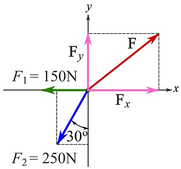
Use the scalar formulation. Determine the magnitudes of the components of the known forces by decomposing them into their Cartesian components.
![\[\begin{split}\bold F_1&=\bold F_{1x} + \bold F_{1y}\\&\implies F_{1x}=150\text { N}\leftarrow,\qquad F_{1y}=0\text { N}\\\bold F_2&=\bold F_{2x} + \bold F_{2y}\\&\implies F_{2x}=250\sin30^\circ\text { N}\leftarrow, \qquad F_{2y}=250\cos30^\circ\text { N}\downarrow\end{split}\]](https://engcourses-uofa.ca/wp-content/ql-cache/quicklatex.com-ee2dc3a36370e50af16eb2eef5f90ce1_l3.png "Rendered by QuickLaTeX.com")
Involve the unknown force in the equations of equilibrium by the magnitudes and of its components and . Note that and are assumed in the positive directions of the Cartesian axes.
Write the equilibrium equations. The Cartesian axes set the positive direction for the equilibrium equations.
![\[\begin{split}\overset{+}{\rightarrow}\ \sum F_x&=0 \implies F_x-150-250\sin 30^\circ=0 \\+\uparrow\ \sum F_y&=0\implies F_y+0-250\cos 30^\circ=0\end{split}\]](https://engcourses-uofa.ca/wp-content/ql-cache/quicklatex.com-a27d1b490f52ac491a368d3db3cfc204_l3.png "Rendered by QuickLaTeX.com")
leading to,
![\[\begin{cases}F_x=150+250\sin 30^\circ=275\text { N} \rightarrow \\F_y=250\cos 30^\circ=216.5\text { N} \uparrow\end{cases}\]](https://engcourses-uofa.ca/wp-content/ql-cache/quicklatex.com-02140f18907512d7c08e69a24d288859_l3.png "Rendered by QuickLaTeX.com")
Graphically demonstrate the components of .
The magnitude of and its angle with the x axis are determined as,
![\[\begin{split}F&=\sqrt{275^2+217^2}=350\text { N}\\\tan \theta&=\frac{216.5}{275}\implies \theta=\arctan (0.79)= 38.3^\circ\end{split}\]](https://engcourses-uofa.ca/wp-content/ql-cache/quicklatex.com-b5bee86b5d1724dfc82c2571468c7787_l3.png "Rendered by QuickLaTeX.com")
The results is the same as the results in Example 5.1.3.
EXAMPLE 5.1.5
Find the force that establishes the equilibrium conditions for the particle subjected to the forces shown.
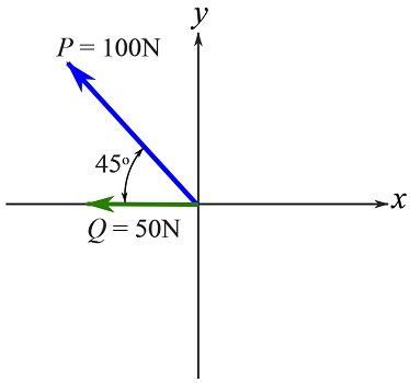
SOLUTION
Use the scalar formulation by following the steps in the previous example.
Magnitudes of the components of the known forces are,
![\[\begin{split}P_x&=100\cos 45^\circ\text{ N}\leftarrow,\qquad P_y=100\sin 45^\circ\text{ N}\uparrow\\Q_x&=50\text{ N}\leftarrow,\qquad Q_y=0\text{ N}\end{split}\]](https://engcourses-uofa.ca/wp-content/ql-cache/quicklatex.com-e28eb04147fc7c87d2a85b93fa24f01a_l3.png "Rendered by QuickLaTeX.com")
You can assume that positive directions for the components of the unknown force as shown in the figure below.
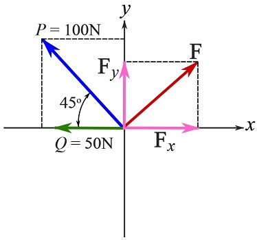
Write the equations of equilibrium and solve for and .
![\[\begin{split}\overset{+}{\rightarrow}\ &\sum F_x=0 \implies -100\frac{\sqrt{2}}{2}-50+F_x=0\\+\uparrow\ &\sum F_y=0\implies 100\frac{\sqrt{2}}{2}+F_y=0\\\end{split}\]](https://engcourses-uofa.ca/wp-content/ql-cache/quicklatex.com-c19e859e9bb3842e89023ebcc8750ef4_l3.png "Rendered by QuickLaTeX.com")
Therefore (by solving the linear system of equations),
![\[\begin{split}F_x= 120.7\text { N}&\implies F_x= 120.7\text { N}\rightarrow\\F_y= -70.7 \text { N}&\implies F_y= 70.7 \text { N}\downarrow\end{split}\]](https://engcourses-uofa.ca/wp-content/ql-cache/quicklatex.com-71eae630100832376e6cca159fde8892_l3.png "Rendered by QuickLaTeX.com")
Note how the signs of the magnitudes imply their corresponding force component directions (represented by the small arrows). Observe that  is reported as
  because should be positive.
Graphically demonstrate the components of .
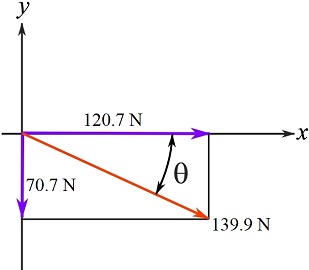
The magnitude of and its angle with the x axis are determined as,
![\[\begin{split}F&=\sqrt{120.7^2+70.7^2}=139.9\text { N}\\\tan\theta&=\frac{F_x}{F_y}=\frac{70.7}{120.7}\implies \theta=30.4^\circ\end{split}\]](https://engcourses-uofa.ca/wp-content/ql-cache/quicklatex.com-793f05a8fc7b4ee3442b19e23ff38afb_l3.png "Rendered by QuickLaTeX.com")
As demonstrated by the above examples, using the magnitudes of the components of the unknown force in the equations facilitates solving the equations of equilibrium, therefore, this approach is recommended.
Remark: the final answer to the equations of equilibrium does not depend on the assumed direction of the unknown force(s). If a wrong direction (or sense of direction) is assumed, the magnitude of the force(s) will turn out to be negative and therefore the sense of direction should be switched to obtain the true direction.
Equations of equilibrium for spatial force system (three dimensions)
In three dimensions, the three force components exist for a force are usually expressed in CVN, i.e.,
![\[\bold F=F_x\bold i + F_y\bold j + F_z\bold k\]](https://engcourses-uofa.ca/wp-content/ql-cache/quicklatex.com-c0a67bf6d3ca4aadde5e8403b6cb32a6_l3.png "Rendered by QuickLaTeX.com")
where , , and  are the scalar components whose their signs are determine based on the direction of , and
  relative to
  ,
,  , and
, and  .
.
Based on CVN, the equations of equilibrium of a particle in three dimensions are obtained by extending Eq. 5.2 to three dimensions as,
![\[\bold F_R=\sum \bold F_x + \sum \bold F_y + \sum \bold F_z =\bold 0\]](https://engcourses-uofa.ca/wp-content/ql-cache/quicklatex.com-ef3bf3c3af80c72136cbed61f2a28751_l3.png "Rendered by QuickLaTeX.com")
Written in CVN,
![\[\bold F_R = \sum F_x\bold i + \sum F_y\bold j + \sum F_z\bold k=\bold 0\]](https://engcourses-uofa.ca/wp-content/ql-cache/quicklatex.com-6b512a2e4954540c1d88ada97d8b4220_l3.png "Rendered by QuickLaTeX.com")
which is satisfied if,
(5.4) ![\[\begin{split}\sum F_x&=0 \\\sum F_y&=0 \\\sum F_z&=0\end{split}\]](https://engcourses-uofa.ca/wp-content/ql-cache/quicklatex.com-de49ac0cb215266545253b9b9c5ec18b_l3.png "Rendered by QuickLaTeX.com")
Equation 5.4 indicates that a particle is in equilibrium if and only if the sum of the scalar components of the forces acting on the particle is zero in each direction.
The equations of equilibrium in three dimensions can be solved for up to three unknowns in a system of forces acting on a particle. An unknown force (vector) has four unknowns, its magnitude and three coordinate direction angles The correlation between the three coordinate direction angles provides an extra equation to be used (see Section 2.4 for details),
![\[\cos^2\alpha + \cos^2\beta + \cos^2\gamma=1\]](https://engcourses-uofa.ca/wp-content/ql-cache/quicklatex.com-bedd731fa847b4a1fe07f86dbfec9102_l3.png "Rendered by QuickLaTeX.com")
In some problems, the direction of the unknown force (or forces) is known and only the magnitude and sense of direction must therefore be determined. These type of problems are solved by initially assuming a sense of direction for the unknown force (or forces) and solving for the magnitude. If the solution leads to a negative value for the magnitude, the assumed sense of direction of the force has to be switched.
EXAMPLE 5.1.6
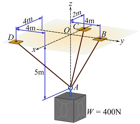
A power speaker is hung from the ceiling with three cables as shown. If the weight of the power speaker is 400N, determine the magnitudes of the cable forces.
SOLUTION
Since the cables become concurrent at the center of the ring connected to the hung power speaker, their forces are also concurrent. Therefore, the ring can be modeled as a particle. Modeling the ring as a particle, follow these steps to determine the cable forces.
Draw the FBD of the ring.
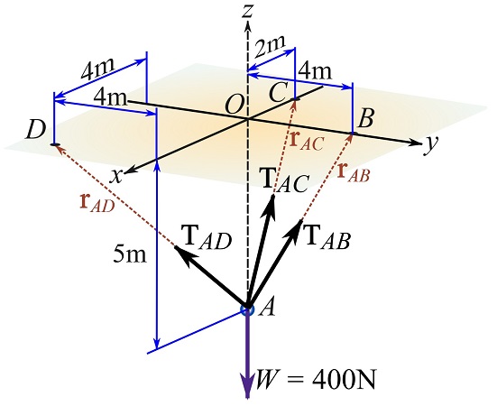
Because a cable can only resist tension, the cable forces pull on the ring and therefore the sense of direction of each cable force is known. The following figure shows the FBD.
Express the forces in CVN.
The direction of a cable force is along the the position vector connecting two points of a cable. Therefore, you can use the position vectors  ,
,  , and
, and  as shown in the figure above.
Using the coordinates of the points  ,
,  ,
,  ,
,  , write,
![\[\begin{split}\bold r_{AB}&=(0-0)\bold i + (4-0)\bold j + (0-(-5))\bold k= \{0\bold i + 4\bold j +5\bold k\}\text m \\\bold r_{AC}&= (-2-0)\bold i + (0-0)\bold j + (0-(-5))\bold k= \{-2\bold i + 0\bold j +5\bold k\}\text m\\\bold r_{AD}&= (4-0)\bold i + (-4-0)\bold j + (0-(-5))\bold k= \{4\bold i -4\bold j +5\bold k\}\text m\end{split}\]](https://engcourses-uofa.ca/wp-content/ql-cache/quicklatex.com-921642f11c6030d2c19bf89239b70a7b_l3.png "Rendered by QuickLaTeX.com")
As the sense of direction of , , and are the same as the sense of direction of the forces  ,
,  , and
, and  respectively, you can write,
![\[\begin{split}\bold T_{AB}&=|\bold T_{AB}|\frac{\bold r_{AB}}{|\bold r_{AB}|}=|\bold T_{AB}|\frac{0\bold i + 4\bold j +5\bold k}{\sqrt{4^2 +5^2}}=|\bold T_{AB}|\{0\bold i + 0.625\bold j+0.781\bold k\}\text N\\\bold T_{AC}&=|\bold T_{AC}|\frac{\bold r_{AC}}{|\bold r_{AC}|}=|\bold T_{AC}|\frac{-2\bold i + 0\bold j +5\bold k}{\sqrt{2^2+5^2}}=|\bold T_{AC}|\{-0.371\bold i + 0\bold j+0.929\bold k\}\text N\\\bold T_{AD}&=|\bold T_{AD}|\frac{\bold r_{AD}}{|\bold r_{AD}|}=|\bold T_{AD}|\frac{4\bold i - 4\bold j +5\bold k}{\sqrt{4^2+4^2+5^2}}=|\bold T_{AD}|\{0.530\bold i - 0.530\bold j+0.662\bold k\}\text N\end{split}\]](https://engcourses-uofa.ca/wp-content/ql-cache/quicklatex.com-015e6709b2112244cef228ba33bd8789_l3.png "Rendered by QuickLaTeX.com")
The weight in CVN is  .
.
Write the equations of equilibrium (Eq. 5.4).
![\[\begin{split}\sum F_x &= 0\implies 0|\bold T_{AB}|-0.371|\bold T_{AC}|+0.530|\bold T_{AD}|=0\\\sum F_y &= 0\implies 0.625|\bold T_{AB}|+0|\bold T_{AC}|-0.530|\bold T_{AD}|=0\\\sum F_z &= 0\implies 0.781|\bold T_{AB}|+0.929|\bold T_{AC}|+0.662|\bold T_{AD}|=400\end{split}\]](https://engcourses-uofa.ca/wp-content/ql-cache/quicklatex.com-54896612f767b2de11b4e20c23ae37fc_l3.png "Rendered by QuickLaTeX.com")
which is a system of equations whose unknowns are the magnitudes of the cable forces.
Solve the system of equations for the magnitudes.
Therefore,
![\[|\bold T_{AB}|=127.9\text N,\qquad |\bold T_{AC}|=215.5\text N,\qquad, |\bold T_{AD}|=150.9\text N\]](https://engcourses-uofa.ca/wp-content/ql-cache/quicklatex.com-8feddc820e2b6b2e47039ea30db72783_l3.png "Rendered by QuickLaTeX.com")
The solution of the system of equations led to positive values for the magnitudes of the forces, therefore, the sense of direction of each force has been correctly assumed (as expected).
Caution: in some textbooks, the magnitude of a force (e.g. ) in three dimensions is denoted by a non-bold letter (e.g.  ), as an alternative to using
  (e.g.
(e.g.  ).
).
Videos
Force Equilibrium:
Particle Equilibrium: