
Forces and Moments: Forces
Definition of force
In general, force is perceived as push or pull. Forces arise from different sources/causes like gravity, contact forces between bodies, pressure force by fluids on surface of solids, friction forces, electrostatic forces on charged particles, etc.
Physically, force has a magnitude and a direction in the space, and therefore, it is a vector quantity called the force vector. In this regard, the terms force and force vector are equivalent. Calculations regarding forces follow the concepts and methods presented in Chapter 2.
The SI unit of force is Newton (N). A force vector has the dimension  , being equal to
  in the SI unit system (see Section 1.2). The direction of a force vector can be expressed using a unit vector. This unit vector shows the direction in the (geometrical) space. We can also have a graphical representation of a force vector. This graphical representation is by the means of an arrow as discussed in Section 2.2. The length of an arrow representing a force vector can be proportional to the vector’s magnitude following some scale.
Denoting a force vector as  , we can write,
(3.1) ![\[\bold F=|\bold F|\bold u_F \]](https://engcourses-uofa.ca/wp-content/ql-cache/quicklatex.com-9a846a9dc17746317ec4519087f19560_l3.png "Rendered by QuickLaTeX.com")
where  is the magnitude of the force and
  is the unit vector expressing the direction of . Note that
  has the unit of Newton, and the unit vector has no dimension and unit. Equation 3.1 readily implies that,
(3.2) ![\[\bold u_F = \frac{\bold F}{|\bold F|} \]](https://engcourses-uofa.ca/wp-content/ql-cache/quicklatex.com-5b11b3319212f1d32417bb95764e4f92_l3.png "Rendered by QuickLaTeX.com")
Line of action of a force. The line of action of a force or a force vector is a line that is collinear with the force vector (arrow representing the force).
Like any vector, a force vector can be resolved into its Cartesian components using the CVN,
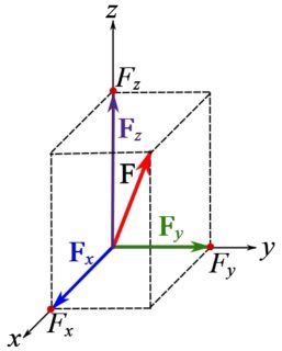
(3.3) ![\[\bold F = F_x\bold i + F_y\bold j + F_z\bold k \]](https://engcourses-uofa.ca/wp-content/ql-cache/quicklatex.com-ec08b28326881ebfa61d09c8f52ec5ee_l3.png "Rendered by QuickLaTeX.com")
where  are the scalar components.
A graphical representation of in the Cartesian frame is shown in Fig. 3.1.
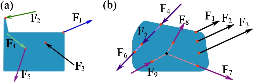
We say a body is subjected to a force (or a system of forces), or a force acts on a body. This expresses the fact that a force is acting or exerted at a particular location of the body. Therefore, the location at which a force vector is acting is deterministically important and not arbitrary. This is graphically demonstrated by drawing the force vector with its tail or head touching the point at which the force acts (Fig. 3.2a). Depending on the tail or the head of the vector touching the point, this representation may also imply a sense of pull or push by the force (Fig 3.2a).
Parallel forces. Two or more forces are called parallel if their line of actions are parallel. For example,  ,
,  , and
, and  are parallel in Fig. 3.2b.
Collinear forces. Two or more forces are called collinear if they share the same line of action. Consequently, collinear forces are parallel. However, parallel forces may not be collinear. For example,  ,
,  , and
, and  are collinear in Fig. 3.2b.
Concurrent forces. Two or more forces are called concurrent if their lines of action intersect at a common point. For example,  ,
,  , and
, and  are concurrent in Fig. 3.2b.
a force always accompanies a point at which the force is acting.
Concentrated force. In reality, forces are continuously distributed over areas. For example, we perceive and feel that the ground reaction force due to our weight is distributed on the soles of our feet; we do not feel a sharp feeling of a force there. In fact, all forces in nature are distributed, and there is no force concentrated at (or acting on) a point. However, we idealize or approximate a distributed force by a concentrated force. This idealization is performed when the area on which the load is distributed is relatively small compared to the size of the body.
Resultant force
Let  be a system of
  forces (set of forces), their resultant or the resultant force
  is a vector sum over the forces (see Section 2.4),
(3.4) ![\[ \bold F_R = \bold F_1 + \bold F_2 + \dots + \bold F_n=\sum_{i=1}^n\bold F_i \]](https://engcourses-uofa.ca/wp-content/ql-cache/quicklatex.com-5294438e6f25e335313d7efe8e28e94d_l3.png "Rendered by QuickLaTeX.com")
Remark: vector addition of forces does not depend on the location of forces on a body.
The calculation procedure of resultants of forces can be presented separately for coplanar and spatial force systems.
Coplanar force systems (Two-dimensions)
A coplanar force system or a system of coplanar forces is a set of forces with their lines of action all in the same plane. Therefore, each force in a coplanar force system has two Cartesian components in a plane Cartesian coordinate system as presented in Section 2.4.2. With  and
and  being the axes of a Cartesian frame, a planar is written in CVN as,
(3.5a) ![\[\bold F = \bold F_x + \bold F_y = F_x\bold i + F_y\bold j \]](https://engcourses-uofa.ca/wp-content/ql-cache/quicklatex.com-f707b1bf0ea407699039c98c0c364384_l3.png "Rendered by QuickLaTeX.com")
The the following equations hold for the magnitude, and scalar components of planar forces,
(3.5b) ![\[F=|\bold F| = \sqrt {F_x^2 + F_y^2},\quad \tan \theta=\frac{|F_y|}{|F_x|}\]](https://engcourses-uofa.ca/wp-content/ql-cache/quicklatex.com-57f3a9407a8644388f25bc01afa73efd_l3.png "Rendered by QuickLaTeX.com")
where  is the angle of with the axis as shown in Fig. 3.3.
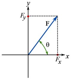
Note that a new notation for the magnitude of (not its components) is defined as being a non-bold capital letter. We will used instead of when denoting the magnitude of a planar force. This labeling approach applies to the two-dimensional calculation of any vectors for simplicity.
To determine the resultant force of a coplanar force system, the equations presented in Sections 2.4.2 and 2.4.3 are implemented. Here, we repeat the equations for a force system.
For a system of coplanar forces  , if each force is expressed in CVN as,
![\[\begin{split} \bold F_1&=F_{1x}\bold i + F_{1y}\bold j\\ \bold F_2&=F_{2x}\bold i + F_{2y}\bold j\\ &\vdots\\ \bold F_n&=F_{nx}\bold i + F_{ny}\bold j \end{split} \]](https://engcourses-uofa.ca/wp-content/ql-cache/quicklatex.com-470598cce4a165eeb676af59cd7a7fee_l3.png "Rendered by QuickLaTeX.com")
the resultant force is determined as,
(3.6a) ![\[\bold F_R = \sum_{i=1}^n\bold F_i = \left(\sum_{i=1}^n F_{ix}\right)\bold i + \left(\sum_{i=1}^n F_{iy}\right )\bold j=(\bold F_R)_x + (\bold F_R)_y\]](https://engcourses-uofa.ca/wp-content/ql-cache/quicklatex.com-83591d17af0f4b5b2835a0970a7be1fc_l3.png "Rendered by QuickLaTeX.com")
which is written in the following concise way,
(3.6b) ![\[ \bold F_R = \sum \bold F = (\sum F_x)\bold i +(\sum F_y)\bold j \]](https://engcourses-uofa.ca/wp-content/ql-cache/quicklatex.com-b97d0267f4cbc5976c79348bca6e5e7a_l3.png "Rendered by QuickLaTeX.com")
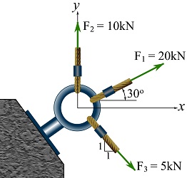
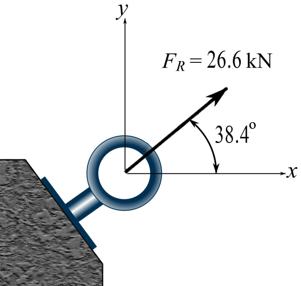
EXAMPLE 3.1.1
Determine the resultant force of the cable forces shown in the figure. Obtain the force vector, its magnitude, and its direction measured from the positive x-axis shown.
SOLUTION
![\[\begin{split}\bold F_1&=\{20\cos 30^\circ \bold i+20\sin 30^\circ\bold j\}=\{17.3\bold i+10.0\bold j\}\text{ kN}\\\bold F_2&=\{0\bold i + 10\bold j\}\text{ kN}\\\bold F_3&=\{5\cos 45^\circ\bold i+5\sin 45^\circ\bold j\}=\{3.5\bold i - 3.5\bold j\}\text{ kN}\\\therefore \bold F_R&=\bold F_1 + \bold F_2 + \bold F_3= \{17.3+0+3.5\}\bold i+\{10.0+10.0-3.5\}\bold j\\&=\{20.8\bold i+16.5\bold j\}\text{ kN}\\\implies F_R&=|\bold F_R|=\sqrt{20.8^2+16.5^2}=26.6 \text{ kN}\\\\ \theta&=\arctan\frac{16.5}{20.8}=38.4^\circ\end{split}\]](https://engcourses-uofa.ca/wp-content/ql-cache/quicklatex.com-df47e7660537985d3fe705b30d5487ee_l3.png "Rendered by QuickLaTeX.com")
Spatial force systems (three-dimensions)
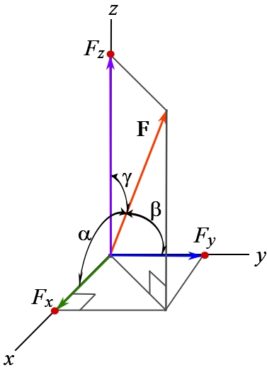
A spatial system of forces, is a general force system with forces not necessarily lying in one plane. A spatial force can be represented by three Cartesian components as formulated in Section 2.4.4. With x, y and z being the axes of a Cartesian frame, is written in CVN as,
(3.7a) ![\[\bold F = \bold F_x + \bold F_y + \bold F_z= F_x\bold i + F_y\bold j + F_z\bold k \]](https://engcourses-uofa.ca/wp-content/ql-cache/quicklatex.com-847436d96ef68065187ac905110a5055_l3.png "Rendered by QuickLaTeX.com")
The following equations hold for the magnitude, and scalar components of the force,
(3.7b) ![\[\begin{split}|\bold F|&=\sqrt{F_x^2 +F_y^2 +F_z^2}\\\cos \alpha=\frac{F_x}{|\bold F|} \quad &\cos \beta=\frac{F_y}{|\bold F|} \quad \cos \gamma=\frac{F_z}{|\bold F|} \end{split}\]](https://engcourses-uofa.ca/wp-content/ql-cache/quicklatex.com-7aaebd424753a6b2420bbdb2b5fb6779_l3.png "Rendered by QuickLaTeX.com")
where  are the coordinate direction angles as shown in Fig. 3.4.
The resultant force of a system of spatial forces containing  expressed in CVN is,
(3.8) ![\[ \bold F_R = \sum \bold F = (\sum F_x)\bold i +(\sum F_y)\bold j +(\sum F_z)\bold k \]](https://engcourses-uofa.ca/wp-content/ql-cache/quicklatex.com-4ee0c00bdfc295cd193e2251f1816482_l3.png "Rendered by QuickLaTeX.com")
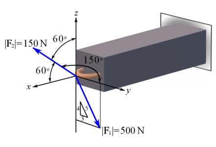
EXAMPLE 3.1.2
A box beam is subjected to the forces as shown. Express each force in CVN and determine the magnitude and coordinate direction angles of the resultant force.
SOLUTION
To express the , the scalar components of are determined and we write  .
.
![\[\begin{split}F_{1x} &= 0 \rm{N}\\F_{1y} &= 500 \frac{3}{5} = 300 \rm{N}\\F_{1z} &= -500 \frac{4}{5} = -400 \rm{N}\\\implies \bold F_1&=\{0\bold i + 300\bold j - 400\bold k\}\rm N\end{split}\]](https://engcourses-uofa.ca/wp-content/ql-cache/quicklatex.com-bbfd62379924a36425ae7e5523ec66a5_l3.png "Rendered by QuickLaTeX.com")
And for ,
![\[\begin{split}F_{2x} &= 150\cos(60^\circ)= 75\rm{N}\\F_{2y} &= 150\cos(150^\circ)= -130\rm{N}\\F_{2z} &= 150\cos(60^\circ)= 75\rm{N}\\\implies \bold F_2&=\{75\bold i -130\bold j +75\bold k\}\rm N\end{split}\]](https://engcourses-uofa.ca/wp-content/ql-cache/quicklatex.com-e605f4a95514e2b3ee2ae499bcdd6dbc_l3.png "Rendered by QuickLaTeX.com")
Therefore,
![\[\bold F_R=\bold F_1 + \bold F_2= (0+75)\bold i + (300-130)\bold j+ (- 400+75)\bold k= \{75\bold i + 170\bold j -325\bold k\}\rm N\]](https://engcourses-uofa.ca/wp-content/ql-cache/quicklatex.com-e94fc1a2de14ed4f174ebf6dce7cf561_l3.png "Rendered by QuickLaTeX.com")
Leading to,
![\[|\bold F_R|=\sqrt{75^2+170^2+325^2}= 374 \rm N\]](https://engcourses-uofa.ca/wp-content/ql-cache/quicklatex.com-74b64ae71f1c752d66e9643cca0c35cb_l3.png "Rendered by QuickLaTeX.com")
The direction angles of are,
![\[\begin{split}\cos \alpha &= \frac{75}{374.4} \Rightarrow \alpha = 78.5^\circ \\\cos \beta &= \frac{170}{374.4} \Rightarrow \beta = 63.0^\circ \\\cos \gamma &= \frac{-325}{374.4} \Rightarrow \gamma = 150.1^\circ\end{split}\]](https://engcourses-uofa.ca/wp-content/ql-cache/quicklatex.com-10ce2b6de04a254ac11d23f0ce160695_l3.png "Rendered by QuickLaTeX.com")
Force directed along a line
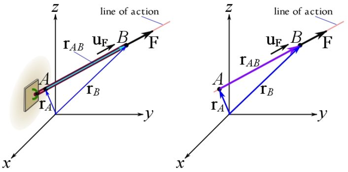
In many problems, a force is directed along a line-shape physical object or structure like a cable or a bar. In such a case, the line of action of the force is collinear with the direction of the object (Fig. 3.5). The line of action of the force is, therefore, determined by two points along the structure.
To determine a force directed along a line, we initially choose (or consider a given) a Cartesian coordinate system. Choosing a point as the coordinate system origin (if not given) is arbitrary, however, we should try to wisely choose a point that will simplify the calculations. Then, two points, say A and B, on the line of action or the object are identified. These are points with known coordinates or points that their coordinates are easy enough to calculate (Fig. 3.5). Considering the position vectors of A and B, we find the vector  as,
as,
(3.9) ![\[\bold r_{AB}=\bold r_B-\bold r_A=(x_B-x_A)\bold i+(y_B-y_A)\bold j+(z_B-z_A)\bold k \]](https://engcourses-uofa.ca/wp-content/ql-cache/quicklatex.com-5ee1bb026f7044eb281c22443d5877c9_l3.png "Rendered by QuickLaTeX.com")
The unit vector is obtained by normalizing by its magnitude (length),  , assuming AB is the direction of the force. Consequently, the force vector can be written as,
(3.10) ![\[\bold F=|\bold F|\bold u_F=|\bold F|\frac{\bold r_{AB}}{|\bold r_{AB}|}=|\bold F|\frac{\bold (x_B-x_A)\bold i+(y_B-y_A)\bold j+(z_B-z_A)\bold k}{\sqrt{(x_B-x_A)^2+(y_B-y_A)^2+(z_B-z_A)^2}}\]](https://engcourses-uofa.ca/wp-content/ql-cache/quicklatex.com-acde48ea16f83b6cc215a02452ab2566_l3.png "Rendered by QuickLaTeX.com")
As shown in Fig. 3.5, the graphical representation of , and  are collinear. Note that has the dimension of force, has the dimension of length, and the unit vector has no dimension. Despite having different dimensions and units, all the vector quantities can be graphically shown in one Cartesian coordinate system (frame).
The following interactive tool illustrates obtaining a force vector directed along a line with two known points.
EXAMPLE 3.1.3
Determine the magnitude and coordinate direction angles of the resultant force.  ,
,  and
and  .
.
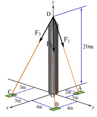
SOLUTION
The following position vectors are needed to determine the directions of the forces.
![\[\begin{split}\bold u_{DA} &= \frac{\bold r_A - \bold r_D}{| \bold r_{DA} |} = \frac{-3 \bold i + 2 \bold j - 20 \bold k}{\sqrt{3^2 + 2^2 + 20^2}}\\\bold u_{DB} &= \frac{\bold r_B - \bold r_D}{| \bold r_{DB} |} = \frac{4\bold i + 4 \bold j - 20 \bold k}{\sqrt{4^2 + 4^2 + 20^2}}\\\bold u_{DC} &= \frac{\bold r_C - \bold r_D}{| \bold r_{DC} |} = \frac{5 \bold i - 3 \bold j - 20\bold k}{\sqrt{5^2 + 3^2 + 20^2}}\end{split}\]](https://engcourses-uofa.ca/wp-content/ql-cache/quicklatex.com-a185cab6860f5eabbbdbc6beed5de39f_l3.png "Rendered by QuickLaTeX.com")
The forces are found as,
![\[\begin{split}\bold F_1 &= |\bold F_1|\bold u_{DA} = 400 \frac{-3 \bold i + 2 \bold j - 20 \bold k}{\sqrt{3^2 + 2^2 + 20^2}} \\&=\{-59.04 \bold i + 39.37 \bold j - 393.65 \bold k\}\rm N\\\bold F_2 &= |\bold F_2|\bold u_{DB} = 200 \frac{4\bold i + 4 \bold j - 20 \bold k}{\sqrt{4^2 + 4^2 + 20^2}} \\&=\{38.49 \bold i + 38.49 \bold j - 192.45 \bold k\} \rm N\\\bold F_3 &= |\bold F_3|\bold u_{DC}= 300 \frac{5 \bold i - 3 \bold j - 20\bold k}{\sqrt{5^2 + 3^2 + 20^2}}\\&=\{72 \bold i - 43.20 \bold j - 288 \bold k\} \rm N\end{split}\]](https://engcourses-uofa.ca/wp-content/ql-cache/quicklatex.com-0553c70d40142860f71e4c6760169558_l3.png "Rendered by QuickLaTeX.com")
Therefore, the resultant force is,
![\[\begin{split}\bold F_R &= \bold F_1 + \bold F_2 + \bold F_3\\&=(-59.04 + 38.49 + 72 )\bold i + (39.37 + 38.49 - 43.2)\bold j + (-393.65 - 192.45 - 288) \bold k \\&=\{51.45 \bold i +34.66 \bold j - 874.10 \bold k\} \rm N\\|\bold F_R| &= 876.72 \rm N\end{split}\]](https://engcourses-uofa.ca/wp-content/ql-cache/quicklatex.com-4aa94e1c23a69e8a88607d00a02113df_l3.png "Rendered by QuickLaTeX.com")
The coordinate direction angles  ,
,  , and
, and  (the angls of the resultant force with , , and
  axes respectively) are, therefore, determined as,
![\[\begin{split}\alpha &= \arccos (\frac{51.45}{876.72}) = 86.64^{\circ} \\\beta &= \arccos (\frac{34.66}{876.72}) = 87.70^{\circ} \\\gamma &= \arccos (\frac{-874.10}{876.72}) = 175.94^{\circ}\end {split}\]](https://engcourses-uofa.ca/wp-content/ql-cache/quicklatex.com-7d3a3734315785ebc54e15c38bbe1998_l3.png "Rendered by QuickLaTeX.com")
Context: Force directed along a Line
- There is a relationship between position vectors (e.g. member length and angles) and force vectors (e.g. force carried by a member).
- In two dimensional systems, simple trigonometric rules can relate vector components and the angle between vectors. This approach is much more complicated in 3-D systems, so another approach is used instead: dot products.
- Force directed along a line is most easily visualized in cables but occurs in many other members (such as columns, struts, and truss members).
- Engineers select member start and end points based on many factors (e.g. aesthetics, materials, ease of construction) but the most important factor is optimizing how force is carried through the member. For instance, in a system supported by many cables, engineers may proportion cable start and end points to ensure that each cable carries approximately the same forces under the expected loads.
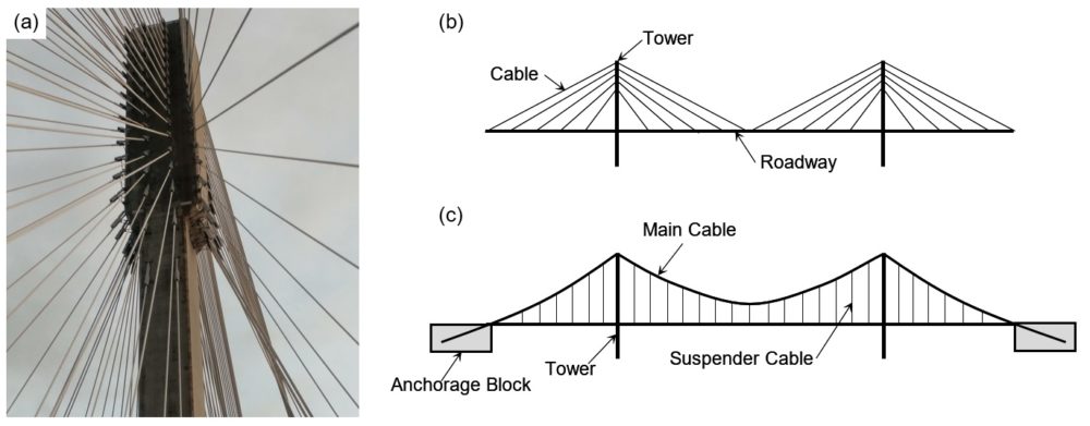
Applications: Why is force along a line important?
The Port Mann Bridge between Surrey and Coquitlam (Vancouver area) opened in 2012 and has one of the longest spans of a cable stayed bridge in North America (470 m) (Fig. 3.6a). To support the roadway, dozens of steel cables connect to one of two large reinforced concrete towers.
Engineers need to consider how much force is carried in each cable to ensure that the tower is not excessively loaded on one side (which would cause the tower to bend or twist). Since each cable acts at a different angle, engineers used force along a line concepts to determine the force in each cable and evaluate if the tower is loaded evenly and ensure that no cables are overloaded (i.e. at risk of snapping). For added complexity, engineers also need to account for how the cables deform (i.e. stretch) when they are under load to ensure they share loads as designed. Deformations are discussed in future courses.
Note that cable stayed bridges are commonly mistaken as suspension bridges. In cable stayed bridges, cables are connected directly between the roadway and the supporting towers (Fig. 3.6b) while suspension bridges (e.g. Golden Gate Bridge) have relatively small vertical cables (‘suspenders’) that transfer loads (weight of road and the traffic) into large curved cables that rest on top of towers and are anchored (held) to the ground (usually via giant concrete anchorage blocks) at either end of the bridge.
Force component using dot product
The component of a force along an arbitrary axis can be determined using the dot product. Let be a force and l an axis with its positive direction defined by a unit vector  as shown in Fig. 3.7. Then, the component of along l is denoted by
  and determined by the orthogonal projection of onto l. Using the dot product to formulate the orthogonal projection (see Chapter 2), is calculated as,
(3.11) ![\[\bold F_u=(\bold F\cdot\bold u)\bold u \]](https://engcourses-uofa.ca/wp-content/ql-cache/quicklatex.com-089588b65e90be43310501f88c618366_l3.png "Rendered by QuickLaTeX.com")
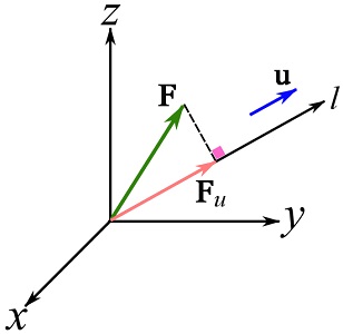
Note that  is the scalar component of along the l axis. Therefore, we can write,
![\[\bold F_u=F_u\bold u\]](https://engcourses-uofa.ca/wp-content/ql-cache/quicklatex.com-0d484143367cbf4b14a0125a5b1916ff_l3.png "Rendered by QuickLaTeX.com")
EXAMPLE 3.1.4
Consider the flagpole shown in the figure. The pole is 15 meters high and stabilized by a cable/rope as shown. Due to the wind, a tension force with a magnitude of  develops in the cable. Determine the force developed along the pole.
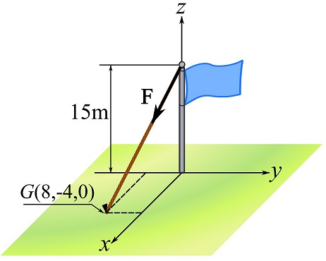
SOLUTION
1- determine the position vector  .
.
![\[\bold r_{PG} = \bold r_{OG}-\bold r_{OP} = 8\bold i - 4\bold j -15 \bold k\]](https://engcourses-uofa.ca/wp-content/ql-cache/quicklatex.com-5494c8b74c579a57a9964f0870ed5c47_l3.png "Rendered by QuickLaTeX.com")
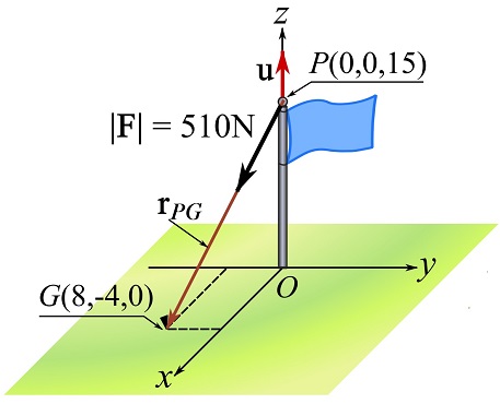
2- Find in CVN.
![\[\begin{split}|\bold r_{PG}|&= \sqrt {8^2 + 4^2 +15^2} = 17.46 \text{ m}\\\bold F &= |\bold F|\frac{\bold r_{PG}}{|\bold r_{PG}|}=510 \frac{8\bold i - 4\bold j -15\bold k}{17.46}\text{N}\\\implies \bold F &=\{234\bold i -117\bold j -438\bold k\}\text {N}\end{split}\]](https://engcourses-uofa.ca/wp-content/ql-cache/quicklatex.com-b908c2d0bbfa57d912a972d9382c6cda_l3.png "Rendered by QuickLaTeX.com")
3- Project onto the z axis.
i) Find the unit vector on z axis.
![\[\bold u=0\bold i + 0\bold j + 1 \bold k\]](https://engcourses-uofa.ca/wp-content/ql-cache/quicklatex.com-566de4e42441c5580f068fd703842448_l3.png "Rendered by QuickLaTeX.com")
ii)
![\[\bold F_z = (\bold F\cdot\bold u)\bold u=\left( (234)(0)+(-117)(0)+(-438)(1)\right ) \bold u= -438\bold u \text { N}\]](https://engcourses-uofa.ca/wp-content/ql-cache/quicklatex.com-01e8adf8a969e9cb6bd295f74825476e_l3.png "Rendered by QuickLaTeX.com")
where  indicates that in in the opposite direction of .
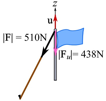
As in this example  coincidentally, we can write
  .
.