
Internal Forces: Shear and moment equations and their diagrams
The internal forces and couple moments in a loaded beam vary along a beam due to the loading conditions (e.g. number of external forces and their distances to the location of the internal forces) are different for different sections of the beam. Consequently, the values of the internal forces and couple moments along a beam must be known for a beam design. For example, maximum values of the shear force and bending moment and their locations along a beam are needed during a beam design.
The internal forces and couple moment acting at any point along the axis of a beam can be determined by the method of sections. In this regard, we need to define the section with a reference point, normally from the left end of the beam. Hence, the location of the internal forces of interest is defined by the distance from the left end of the beam to the point of interest denoted by  (Fig. 7.14). Therefore, shear and bending moment at each point become functions of x (and the external forces), i.e.,
![\[N=N(x),\quad V=V(x), \quad M=M(x)\]](https://engcourses-uofa.ca/wp-content/ql-cache/quicklatex.com-227ac3c1a089fe6464f7c75c009c24b6_l3.png "Rendered by QuickLaTeX.com")
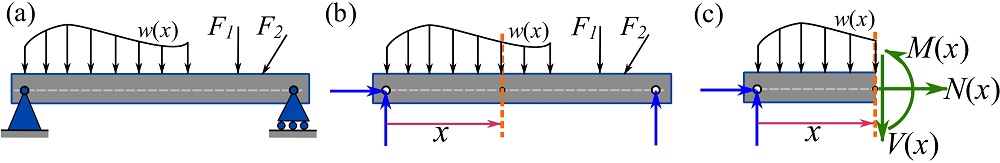
Remark: the signs of the results from  ,
,  , and
, and  refer to the member sign convention (Fig. 7.8, 7.9, and 7.10) because the unknown directions of internal forces are assumed positive according to that sign convention.
Structural beams are commonly long and straight members designed to carry loads mainly perpendicular to their long axes, upward or downward. Perpendicular loads on a beam affect only the shear force and bending moment within the beam, not the axial force In this case, axial force is zero anywhere along the beam.
The functions and and their diagrams (graphs or plots) provide powerful tools for evaluating the values and variations of the shear force and bending moment at any point. The following example demonstrates how to obtain and using the method of sections and plotting them. The and plots are referred to as shear force diagram (SFD) and bending moment diagram (BMD) respectively.
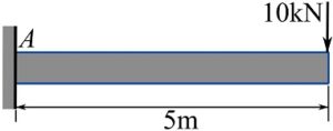
Example 7.2.1
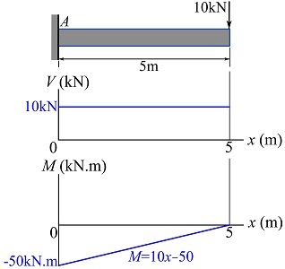
Determine the and for the loaded beam shown in the figure.
SOLUTION
1- Draw the FBD of the beam.
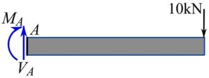
In the FBD, the directions of the unknown force and moment are assumed positive according to the member sign convention.
2- Solve the equations of equilibrium for the support reactions.
![\[\begin{split}\sum F_x&=0\implies A_x=0\\\sum F_y&=0\implies V_A-10=0\implies V_A=10 \text{ kN} \uparrow\\\circlearrowleft{+}\ \sum M_A&=0\implies -M_A-(10)(5)=0\implies M_A=-50\text{ kN.m}\\ &\implies M_A=50 \text{ kN.m} \circlearrowleft\end{split}\]](https://engcourses-uofa.ca/wp-content/ql-cache/quicklatex.com-6c29716016d356236258898069317218_l3.png "Rendered by QuickLaTeX.com")
3- Make a cut in the FBD of the beam at an arbitrary point x meter away from the left end of the beam as shown. Choose one of the two segments for analysis. For instance, the segment chosen is as shown below.
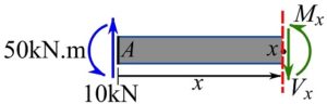
4- Write the equations of equilibrium for the resultant segment and solve for the shear force and bending moment at ,
![\[\begin{split}\sum F_y&=0\implies 10-V_x=0\implies V_x=10 \text{ kN}\\\circlearrowleft{+}\ \sum M_A&=0\implies 50-(V_x)(x)+M_x=0\implies M_x=-50+10x\text{ kN.m}\\ &\implies M_x=10x-50 \text{ kN.m}\end{split}\]](https://engcourses-uofa.ca/wp-content/ql-cache/quicklatex.com-bf8ca279f7ef5b8356fe2fbb73d03602_l3.png "Rendered by QuickLaTeX.com")
Therefore,
![\[\begin{split}V(x)&=10 \text{ kN}\\M(x)&=10x-50 \text{ kN.m}\end{split}\]](https://engcourses-uofa.ca/wp-content/ql-cache/quicklatex.com-eea18e13726dc61ff4e5e6bc016d5ac3_l3.png "Rendered by QuickLaTeX.com")
5- Plot the functions and on x–y plots, with the x axis representing the distance from the left end of the beam, and the y axis representing the values of and . The plot gives a shear force diagram (SFD) and the plot gives a bending moment diagram (BMD).
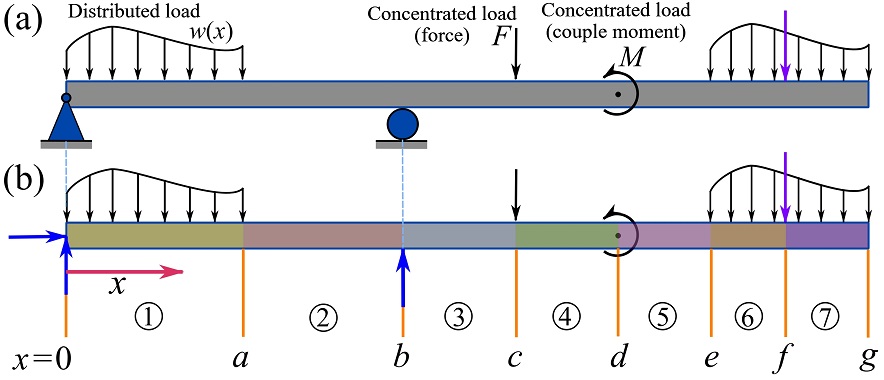
In general, the loading condition on a section between the reference end and the cut will change as the cut moves from one end of the beam to the other, the inputs (external load) to the and will change. Therefore, and may need to be specifically defined for different sections along the axis of a beam. A beam should be divided into sections along its axis (length) at locations where the external load pattern on the FBD of a beam changes. Figure 7.15 shows the sections needed for determining and .
 and are needed.
Example 7.2.2
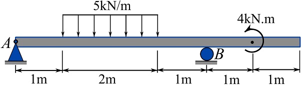
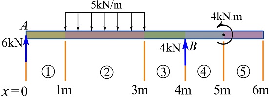
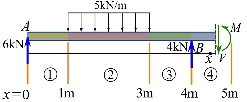
Draw the shear force and bending moment diagrams of the loaded beam shown in the figure.
SOLUTION
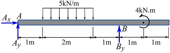
1- Draw the FBD of the beam.
2- Solve the equations of equilibrium for the support reactions.
![\[\begin{split}\sum F_x&=0\implies A_x=0\\\sum F_y&=0\implies -(5)(2)+A_y+B_y=0\\\circlearrowleft{+}\ \sum M_A&=0\implies -(5)(2)(2)+(B_y)(4)+4=0\\\therefore A_y&=6\text{ kN} \uparrow,\quad B_y=4\text{ kN} \uparrow\end{split}\]](https://engcourses-uofa.ca/wp-content/ql-cache/quicklatex.com-0ff7b021030ff54a1bcdc49deee614bd_l3.png "Rendered by QuickLaTeX.com")
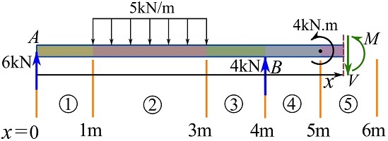
3- Divide the beam (its FBD) into regions based on pattern change of the external loads.
4- In each region, cut at an arbitrary point meter away from the left end of the beam, write the equations of equilibrium, and solve for and .
Arbitrary cut in region 1.
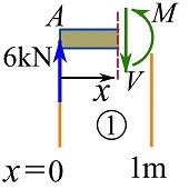
![\[\begin{split}\sum F_y&=0\implies 6-V=0\\\circlearrowleft{+}\ \sum M_{\text{cut}}&=0\implies M-(6)(x)=0\\\end{split}\]](https://engcourses-uofa.ca/wp-content/ql-cache/quicklatex.com-e117018b3deb7bda25bf64c27cab424e_l3.png "Rendered by QuickLaTeX.com")
The notation  means sum of the moments about the point at which the imaginary cut is made.
Therefore,
![\[\begin{matrix}V(x)=6\text{ kN} \quad \text{for } 0< x \le 1\\M(x)=6x\text{ kN.m} \quad \text{for } 0\le x \le 1\\\end{matrix}\]](https://engcourses-uofa.ca/wp-content/ql-cache/quicklatex.com-0132868c5bf9ef715caf3c61e7b7cb59_l3.png "Rendered by QuickLaTeX.com")
Note that the region for does not include  . The reaction force at is a concentrated force under which the shear force has a rapid change (see Example 7.1.2) or mathematically a jump discontinuity. Therefore, the point at which a concentrated force acts should not be included in the region for .
Arbitrary cut in region 2.
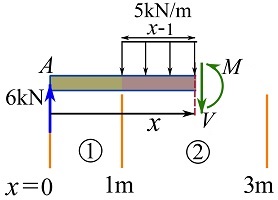
![\[\begin{split}\sum F_y&=0\implies 6-(5)(x-1)-V=0\\\circlearrowleft{+}\ \sum M_{\text{cut}}&=0\implies M + (5)(x-1)(\frac{x-1}{2}) - (6)(x)=0\\\end{split}\]](https://engcourses-uofa.ca/wp-content/ql-cache/quicklatex.com-cbcbdd56b51161f8bddfeb98ac3277ac_l3.png "Rendered by QuickLaTeX.com")
Therefore,
![\[\begin{matrix}V(x)=-5x+11\text{ kN}\quad \text{for } 1\le x \le 3\\M(x)=-2.5x^2+11x-2.5\text{ kN.m}\quad \text{for } 1\le x \le 3\\\end{matrix}\]](https://engcourses-uofa.ca/wp-content/ql-cache/quicklatex.com-2ca6b21db85346194479c2d150dba2d3_l3.png "Rendered by QuickLaTeX.com")
Arbitrary cut in region 3.
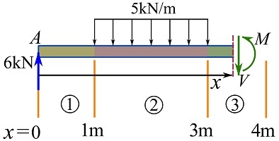
![\[\begin{split}\sum F_y&=0\implies 6-(5)(2)-V=0\\\circlearrowleft{+}\ \sum M_{\text{cut}}&=0\implies M + (5)(2)(x-(1+\frac{2}{2})) - (6)(x)=0\\\end{split}\]](https://engcourses-uofa.ca/wp-content/ql-cache/quicklatex.com-321bf0fe2b3f2a7c6ab7c44edf46a262_l3.png "Rendered by QuickLaTeX.com")
Therefore,
![\[\begin{matrix}V(x)=-4\text{ kN}\quad \text{for } 3\le x < 4\\M(x)=-4x+20\text{ kN.m} \quad \text{for } 3\le x \le 4\end{matrix}\]](https://engcourses-uofa.ca/wp-content/ql-cache/quicklatex.com-035d3cd568c618d5c0f2360a161e71e6_l3.png "Rendered by QuickLaTeX.com")
Note that the region for does not include  . We will see that there will be a jump discontinuity in the diagram of at . The shear force at the location of a concentrated force changes rapidly from one side of the concentrated force to the other side. We just need to know the shear forces on the two sides right next to the concentrated force.
Arbitrary cut in region 4.
![\[\begin{split}\sum F_y&=0\implies 6-(5)(2)+4-V=0\\\circlearrowleft{+}\ \sum M_{\text{cut}}&=0\implies M-(4)(x-4)+(5)(2)(x-(1+\frac{2}{2})) - (6)(x)=0\\\end{split}\]](https://engcourses-uofa.ca/wp-content/ql-cache/quicklatex.com-01701ca7779a7a12c60dbfc06ebd1ed5_l3.png "Rendered by QuickLaTeX.com")
Therefore,
![\[\begin{matrix}V(x)=0 \text{ kN} \quad \text{for } 4< x \le 5\\M(x)=4\text{ kN.m} \quad \text{for } 4\le x < 5\end{matrix}\]](https://engcourses-uofa.ca/wp-content/ql-cache/quicklatex.com-6e5bf0d9db872154431581d0ef9155a5_l3.png "Rendered by QuickLaTeX.com")
Note that the region for does not include  . We will see that there will be a jump discontinuity in the diagram of at . The bending moment at the location of a couple moment changes rapidly from one side of the couple moment to the other side. We just need to know the bending moments on the two sides right next to the couple moment.
Arbitrary cut in region 5.
![\[\begin{split}\sum F_y&=0\implies 6-(5)(2)+4-V=0\\\circlearrowleft{+}\ \sum M_{\text{cut}}&=0\implies M + 4 -(4)(x-4) +(5)(2)(x- (1+\frac{2}{2})) - (6)(x)=0\\\end{split}\]](https://engcourses-uofa.ca/wp-content/ql-cache/quicklatex.com-cd20d7a06b9033c4af116a87bafb1a25_l3.png "Rendered by QuickLaTeX.com")
Therefore,
![\[\begin{matrix}V(x)=0 \text{ kN} \quad \text{for } 5\le x \le 6\\M(x)=0\text{ kN.m} \quad \text{for } 5< x \le 6\end{matrix}\]](https://engcourses-uofa.ca/wp-content/ql-cache/quicklatex.com-b75b7aaf1ab3888f68529be25dad41ee_l3.png "Rendered by QuickLaTeX.com")
5- Plot each functions for each region over the length of the beam.
Collecting the functions over all the regions, you can write,
![\[V(x)=\begin{cases}6\text{ kN}\quad \text{for } 0\le x \le 1 \\-5x+11\text{ kN} \quad \text{for } 1\le x \le 3\\-4\text{ kN}\quad \text{for } 3\le x < 4\\0 \text{ kN} \quad \text{for } 4< x \le 5\\0 \text{ kN} \quad \text{for } 5\le x \le 6\end{cases}\]](https://engcourses-uofa.ca/wp-content/ql-cache/quicklatex.com-1a4debf79d30dcfcb53a9cffd74bb4c9_l3.png "Rendered by QuickLaTeX.com")
and,
![\[M(x)=\begin{cases}6x\text{ kN.m} \quad \text{for } 0< x \le 1\\-2.5x^2+11x-2.5\text{ kN.m} \quad \text{for } 1\le x \le 3\\-4x+20\text{ kN.m} \quad \text{for } 3\le x \le 4\\4\text{ kN.m} \quad \text{for } 4\le x < 5\\0\text{ kN.m} \quad \text{for } 5< x \le 6\end{cases}\]](https://engcourses-uofa.ca/wp-content/ql-cache/quicklatex.com-a25a3915d5f635d5c82922f32113b13b_l3.png "Rendered by QuickLaTeX.com")
The SFD and BMD are as follow.
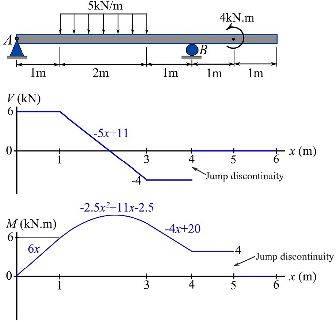
Remark: Any point at which a concentrated force is applied is associated with a jump discontinuity in , this point should not be included in the region over which is being determined. Similarly, Any point at which a couple moment is applied is associated with a jump discontinuity in , this point should not be included in the region over which is being determined.
In the above example, we can visually notice the following effects and changes in the diagrams.
1- A point force creates a jump discontinuity in SFD.
2- A couple moment creates a jump discontinuity in BMD.
3- A discontinuity in the distributed load creates a sudden change of slope (i.e. discontinuity in the slope) in SFD.
4- A point force (also) creates a sudden change of slope in BMD.
These observations are not limited to this problem, but rather they follow general rules that are formally presented in the next section.