
Vectors and their Operations: Dot product
The dot product and its properties
The dot product, also called the scalar product, is an operation that takes two vectors and returns a scalar. The dot product of vectors  and
and  , denoted as
  and read “ dot ” is defined as:
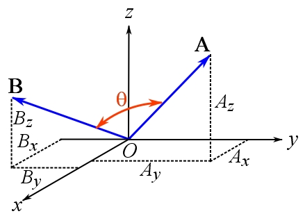
(2.14) ![\[ \bold A\cdot\bold B=|\bold A||\bold B|\cos \theta \]](https://engcourses-uofa.ca/wp-content/ql-cache/quicklatex.com-7e9a4ac105c0bdf4e4e9db3b5e4076f8_l3.png "Rendered by QuickLaTeX.com")
where  is the angle between the two vectors (Fig. 2.24)
From the definition, it is obvious that the result of the dot product is a scalar. The dot product has three properties as follows:
- Commutativity:

- Associativity (scalar multiplication):

- Distributivity:

The proofs of the first two properties are by direct use of the dot product definition (Eq. 2.14). The proof for the third property is by expanding the right hand side of the equation using CVN and using the properties explained below.
Other properties of the dot product
- Dot product of a vector by itself gives its squared magnitude:
 .
. - Dot product of two perpendicular vectors is zero:
 .
. - Dot product by the zero vector is zero:
 .
.
These properties can be easily proved using Eq. 2.14.
Formulation of the dot product using CVN
Let and be two vectors with their scalar components  and
and  . Using CVN, we can write:
![\[ \begin{split} \bold A\cdot \bold B&=(A_x\bold i +A_y\bold j+A_z\bold k )\cdot(B_x\bold i +B_y\bold j+B_z\bold k)\\ &\text{by the distributivity property}\\ &=A_xB_x(\bold i\cdot \bold i)+A_xB_y(\bold i\cdot \bold j)+A_xB_z(\bold i\cdot \bold k)\\ &+A_yB_x(\bold j\cdot \bold i)+A_yB_y(\bold j\cdot \bold j)+A_yB_z(\bold j\cdot \bold k)\\ &+A_zB_x(\bold k\cdot \bold i)+A_zB_y(\bold k\cdot \bold j)+A_zB_z(\bold k\cdot \bold k) \end{split}\]](https://engcourses-uofa.ca/wp-content/ql-cache/quicklatex.com-7c33e58afadbb4a263aef97cc9766446_l3.png "Rendered by QuickLaTeX.com")
The dot product of the unit vectors, by the dot product properties, are:
![\[ \begin{split} \bold i \cdot \bold i&=\bold j \cdot \bold j=\bold k \cdot \bold k=1\\ \bold i \cdot \bold j&=\bold j \cdot \bold i=\bold i \cdot \bold k=\bold k \cdot \bold i=\bold j \cdot \bold k=\bold k \cdot \bold j=0 \end{split}\]](https://engcourses-uofa.ca/wp-content/ql-cache/quicklatex.com-237f2edc7c2d4616730306e6e168a050_l3.png "Rendered by QuickLaTeX.com")
Therefore,
(2.15) ![\[ \bold A\cdot \bold B=A_xB_x+A_yB_y+A_zB_z \]](https://engcourses-uofa.ca/wp-content/ql-cache/quicklatex.com-cac145452937e93b5abedff47fa02058_l3.png "Rendered by QuickLaTeX.com")
This result expresses that the dot product of two vectors written in their CVN can be obtained by multiplying their corresponding scalar components and summing over these products algebraically. Equation 2.15 indicates that calculating the dot product (Eq. 2.14) does not need the magnitudes of two vectors and the angle between them, if the vectors are expressed in CVN.
Application of the dot product: finding the angle between two vectors
The dot product can be used to find the angle formed between two vectors or two intersecting lines. This is helpful particularly when solving problems in three dimensions. The angle between two vectors is obtained by solving Eq. 2.14 for the angle term:
(2.16) ![\[\begin{split}\theta&=\cos^{-1}(\frac{\bold A\cdot\bold B}{|\bold A||\bold B|})\quad 0^\circ\le \theta\le 180^\circ\\\bold A&\cdot \bold B=A_xB_x+A_yB_y+A_zB_z \end{split}\]](https://engcourses-uofa.ca/wp-content/ql-cache/quicklatex.com-9374e75df3b65963f3572eab1e169040_l3.png "Rendered by QuickLaTeX.com")
The above equation can be manipulated as:
(2.17) ![\[\theta=\cos^{-1}(\frac{\bold A}{|\bold A|}\cdot\frac{\bold B}{|\bold B|})=\cos^{-1}(\bold u_A\cdot\bold u_B)\quad 0^\circ\le \theta\le 180^\circ \]](https://engcourses-uofa.ca/wp-content/ql-cache/quicklatex.com-cffc8fb83a12cdf68d3b8e0931dcaf73_l3.png "Rendered by QuickLaTeX.com")
in which  and
and  are the unit vectors of and respectively. This result naturally states that the angle between two vectors only depends on their directions and not on their magnitudes.
Application of the dot product: orthogonal projection of a vector
In many problems, we need to resolve a vector on a particular line or lines in the space. To be more precise, the component of a vector along a particular direction or axis is to be found. Decomposing a vector onto the Cartesian axes is already demonstrated. In this section, we explain decomposing a vector on a general line in space using the dot product. Using the dot product makes the calculation easier specially in three dimensions.
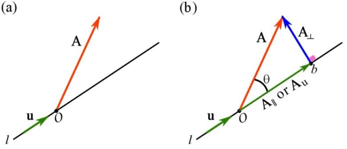
Consider a non-zero vector in the three dimensional space and a line  intersecting the tail of the vector at a point
  (Fig. 2.25a). A unit vector
  is associated with line to assign a direction to the line. In other words, The positive direction of the line is determined by . As demonstrated in Fig. 2.25b, the vector can be written as,
(2.18) ![\[ \bold A =\bold A_{\parallel} + \bold A_{\perp} \]](https://engcourses-uofa.ca/wp-content/ql-cache/quicklatex.com-f0c1095521cd9f70b743fcd6b7458280_l3.png "Rendered by QuickLaTeX.com")
where  is parallel to , and
  is perpendicular to . The symbols
  and
and  denote being parallel and perpendicular respectively.
The vector is referred to as the orthogonal projection (or projection) of onto the line or along the direction of . We denote as  to indicate that is a projection along the direction of .
To obtain , it suffices to note that the vectors , and form a right-angle triangle (Fig. 2.25b). Therefore by the Pythagorean’s theorem  . This inspires us to use Eq. 2.14 and write,
(2.19) ![\[ \begin{split} A_u=|\bold A|\cos \theta&=\bold A\cdot\bold u \\\implies \bold A_u&=A_u\bold u \end{split}\]](https://engcourses-uofa.ca/wp-content/ql-cache/quicklatex.com-a603c0477dd8b3c8ca07d9e2aec22a91_l3.png "Rendered by QuickLaTeX.com")
It should be noted that  is the scalar component of resolved along the direction of . Using the dot product
  to calculate may result in a negative scalar if the angle between
  and are larger than
  . In such a case, the direction of is in the opposite direction of .
The following interactive tool illustrates the orthogonal projection of a vector on the direction defined by a unit vector .
The perpendicular component of can be then obtained by writing,
(2.20) ![\[ \bold A_{\perp}=\bold A-\bold A_u \]](https://engcourses-uofa.ca/wp-content/ql-cache/quicklatex.com-af2cb1c12c2536304790195faa3a85c6_l3.png "Rendered by QuickLaTeX.com")
The magnitude of the perpendicular component can be calculated either by  or
or  .
.
In practice, and can be readily used if  in known, otherwise
  ,
,  , and can be utilized if the components of the vectors in CVN are known.
As a special case, orthogonal projection is used to find the scalar components of a vector, in a Cartesian frame. This is done by writing:
(2.21) ![\[ \begin{split} A_x&=\bold A\cdot \bold i\\ A_y&=\bold A\cdot \bold j\\ A_z&=\bold A\cdot \bold k \end{split}\]](https://engcourses-uofa.ca/wp-content/ql-cache/quicklatex.com-0ed5b636a18650da2b177a3684e2d2b2_l3.png "Rendered by QuickLaTeX.com")
Videos
Dot Product:
Angle Between Vectors:
Orthogonal Projections: