
Centres of Bodies: Centroid
The centers of gravity and mass of a body represent the locations of the concentrated weight and mass (i.e., total weight and total mass), which equal to the original distributed weight and mass of a body (see Sections 3.4 and 3.5 for similar concepts). Now, another step is taken to define the geometric center (or centroid) of a body denoted by  . We used
  for center of gravity and
  for center of mass. The centroid of a body (a volume, a surface, or a line) represents the average location of the constituting or points of the body. We start with defining the centroid of a volume. Then, we define the centroids of surfaces and lines. Note that, the surfaces can be two (flat) or three (curvy) dimensional, and the lines can be two (straight) or three (curvy) dimensional as well.
Centroid of a volume
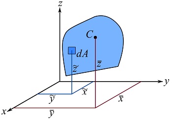
The centroid of a volume of a continuous body (Fig. 9.5) can be calculated as,
(9.14) ![\[\begin{split}\bar x&= \frac{\int_V \tilde x dV}{\int_V dV} = \frac{\int_V \tilde x dV}{V}\\\bar y&= \frac{\int_V \tilde y dV}{\int_V dV} =\frac{\int_V \tilde y dV}{V} \\\bar z&= \frac{\int_V \tilde z dV}{\int_V dV} = \frac{\int_V \tilde z dV}{V} \end{split}\]](https://engcourses-uofa.ca/wp-content/ql-cache/quicklatex.com-e66461b60a08fbb3a29cdb054bb65aca_l3.png "Rendered by QuickLaTeX.com")
where  is the volume of a differential element, the terms
  and
and  denote the coordinates of the centroid of the differential element,
  , and
, and  gives the total volume of the body (Fig. 9.5).
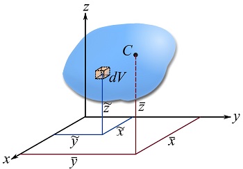
Remark: the centroid of a body does not depend on the coordinate system chosen. It has a fixed location (or distance) with respect to any point of the body. We set a coordinate system merely to calculate the centroid with respect to some point i.e. the origin of the coordinate system.
To implement the integrals in Eq. 9.14, we need to know the location of the centroid of the differential elements in terms of the Cartesian coordinates. Since the differential element are extremely small in size, their centroids are indeed the elements themselves. As discussed in Section 9.1, choosing a Cartesian or a cubic differential element  leads to triple integrals with
  and
and  . Therefore, Eqs. 9.14 takes the following forms in a Cartesian coordinate system with .
(9.15) ![\[\begin{split}\bar x&= \frac{\iiint_V x dxdydz}{\iiint_V dxdydz}=\frac{\iiint_V x dxdydz}{V}\\\bar y&= \frac{\iiint_V y dxdydz}{\iiint_V dxdydz}= \frac{\iiint_V y dxdydz}{V}\\\bar z&= \frac{\iiint_V z dxdydz}{\iiint_V dxdydz}= \frac{\iiint_V z dxdydz}{V} \end{split}\]](https://engcourses-uofa.ca/wp-content/ql-cache/quicklatex.com-09f683363aef2bc799747ef51de30100_l3.png "Rendered by QuickLaTeX.com")
EXAMPLE 9.3.1
Find the centroid of a right rectangular prism with the dimensions as shown.
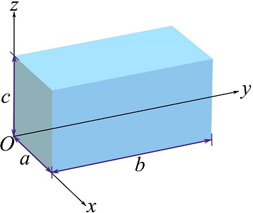
Setting a Cartesian coordinate system and considering a cubic differential element (with a volume of) as shown, calculate the triple integrals in Eqs 9.15.
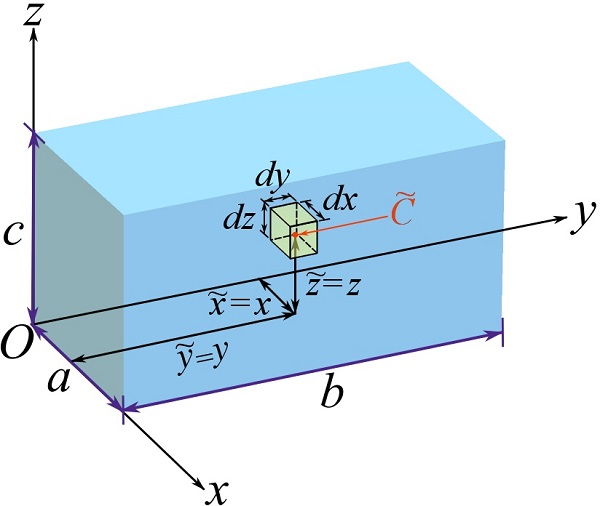
![\[\begin{split}\bar x&=\frac{\iiint_V x dxdydz}{\iiint_V dxdydz}= \frac{1}{abc}\int_0^a\int_0^b\int_0^c x dxdydz=\frac{1}{abc}\int_0^c\left(\int_0^b\left(\int_0^axdx\right)dy\right)dz\\&=\frac{1}{abc}(bc\frac{a^2}{2})=\frac{a}{2}\end{split}\]](https://engcourses-uofa.ca/wp-content/ql-cache/quicklatex.com-1c294d95146c5afeec4f3cdfc4e02959_l3.png "Rendered by QuickLaTeX.com")
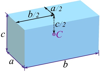
Similarly,
![\[\begin{split}\bar y&=\frac{b}{2}\\\bar z&=\frac{c}{2}\end{split}\]](https://engcourses-uofa.ca/wp-content/ql-cache/quicklatex.com-8fa299962b26b9740904c1abe97593b8_l3.png "Rendered by QuickLaTeX.com")
Therefore, the centroid of a right rectangular prism is as shown,
In many cases, calculating the centroid through triple integrals can be avoided by using differential elements of different convenient shapes other than a prismatic one. The following example shows a case where single-variable integrals are used as a result of using a differential element having the shape of a rectangular prism being differential along only one axis.
EXAMPLE 9.3.2
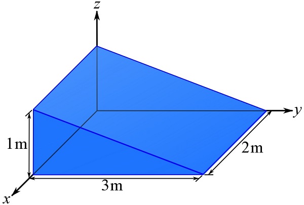
Find the centroid of the solid wedge shown.
SOLUTION
Use volumetric differential element with the shape of a rectangular slice with only one differential side  as shown in the figure below.
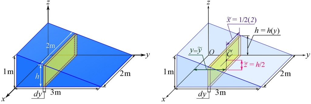
The differential element is  where 2 is the width of the element,
  is the element’s height which linearly varies with
  , and is the differential length of the element. Note that this differential element is regarded as a rectangular cube since is small (approaching zero).
According to Eqs. 9.14, we need to use the coordinates of the centroid of the differential element . From the results of Example 9.3.1, we know that the centroid of a rectangular prism is halfway between all corners. Therefore,  ,
,  as is small, and
  .
.
Using the geometric information of the wedge, we can obtain the height of the differential prism as a function of , i.e.  , we can write,
![\[\begin{split}\bar x&= \frac{\int_V \tilde x dV}{\int_V dV}=\frac{\int_V (1) 2hdy}{\int_V 2hdy}=\frac{\int_0^3 2(-\frac{1}{3}y+1)dy}{\int_0^3 2(-\frac{1}{3}y+1)dy}\\&=1\text{ m}\end{split}\]](https://engcourses-uofa.ca/wp-content/ql-cache/quicklatex.com-7c12e8fd8a2699b7800df2ca638b3aea_l3.png "Rendered by QuickLaTeX.com")
![\[\begin{split}\bar y&= \frac{\int_V \tilde y dV}{\int_V dV}=\frac{\int_V (y) 2hdy}{\int_V 2hdy}=\frac{\int_0^3 2y(-\frac{1}{3}y+1)dy}{\int_0^3 2(-\frac{1}{3}y+1)dy}\\ &=1\text{ m}\end{split}\]](https://engcourses-uofa.ca/wp-content/ql-cache/quicklatex.com-2e62a644682b3f81c0a6423c4ea8e0c4_l3.png "Rendered by QuickLaTeX.com")
![\[\begin{split}\bar z&= \frac{\int_V \tilde z dV}{\int_V dV}=\frac{\int_V (\frac{h}{2}) 2hdy}{\int_V 2hdy}=\frac{\int_0^3 (-\frac{1}{3}y+1)^2dy}{\int_0^3 2(-\frac{1}{3}y+1)dy}\\ &=\frac{1}{3}\text{ m}\end{split}\]](https://engcourses-uofa.ca/wp-content/ql-cache/quicklatex.com-8332a785a5e5ee978cec01a3176f1183_l3.png "Rendered by QuickLaTeX.com")
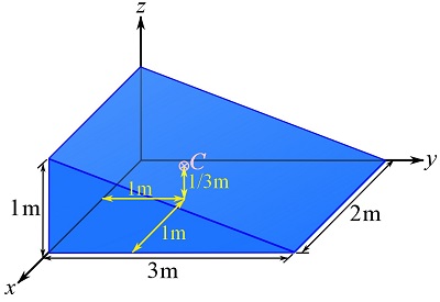
Therefore, the centroid of the wedge is  and it is shown as,
As an alternative, we can consider the following differential element with a differential side  . Solving Eqs. 9.14, we are be able to obtain the same results for the centroid of the wedge.
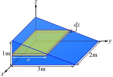
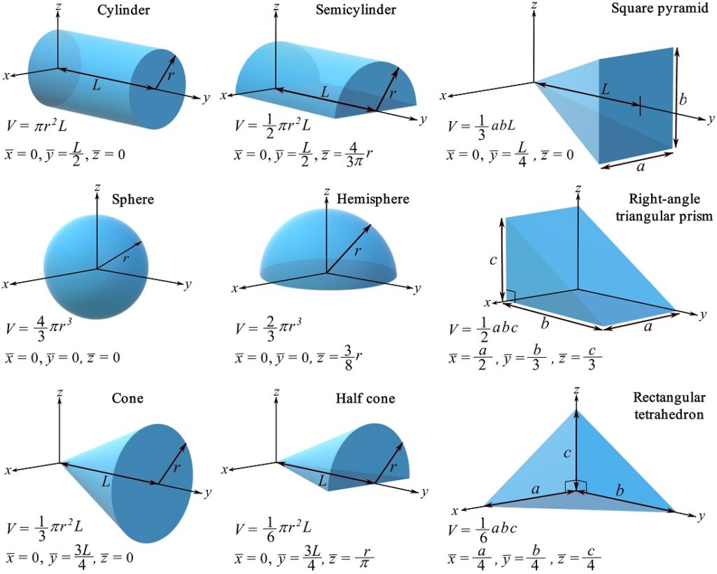
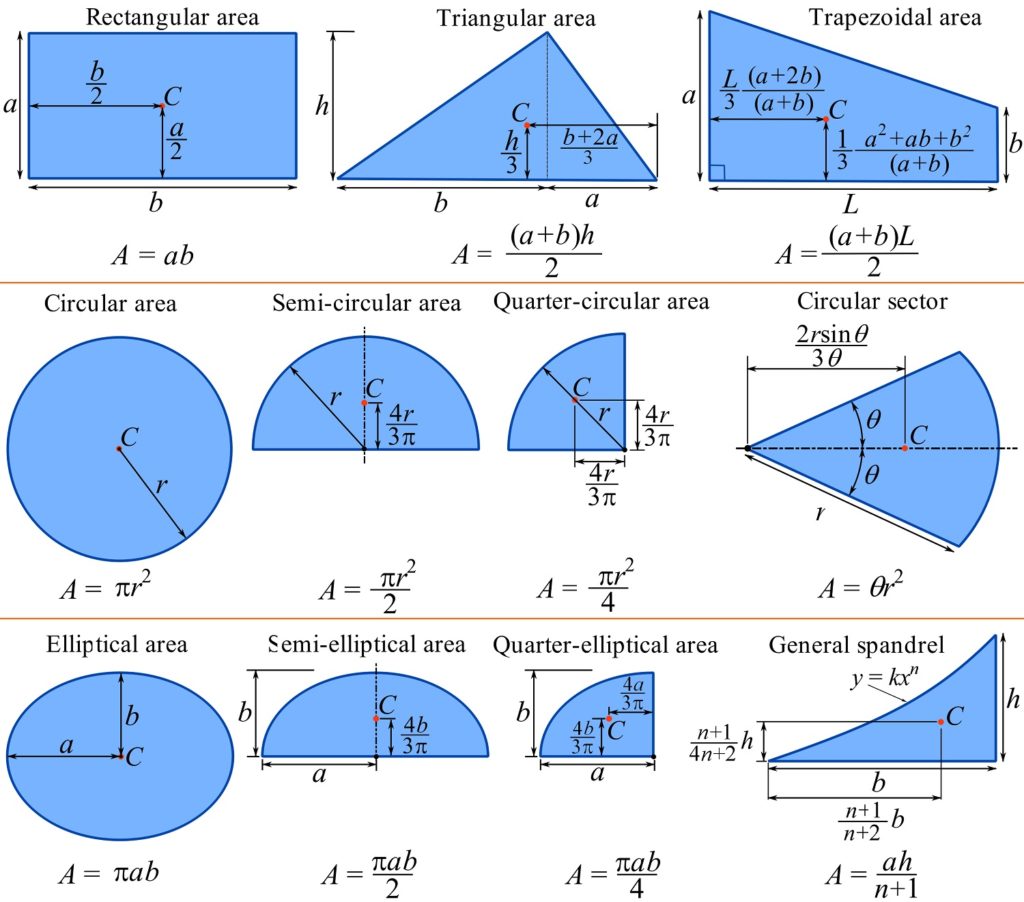
Figure 9.6 demonstrates the volumes and coordinates of centroids of some typical shapes. Note the location of the origin of the coordinate system with respect to which the centroid coordinates are calculated.
Relationship between the centroid, center of mass, and center of gravity of a body
Centroid is a geometric property of a body; the center of mass entails the distribution of the mass of the body in addition to the geometry. The center of gravity brings the effect of the spatial distribution of a gravitational field in to account as well. If a body (or part of a body) is made of a homogeneous material, i.e. having constant specific weight  and density
  , then the locations (or coordinates) of all the three quantities are the same, meaning that,
(9.16) ![\[C=C_m=G\]](https://engcourses-uofa.ca/wp-content/ql-cache/quicklatex.com-03598da81f99ecf8329ec9004bb55978_l3.png "Rendered by QuickLaTeX.com")
Centroid of a surface
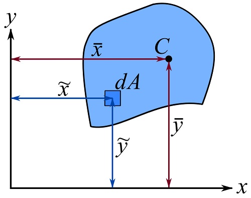
The centroid or geometric center can also be defined for surfaces. The coordinates  of the Centroid of a surface (Fig. 9.7) in the three dimensional space (Fig. 9.7) can be calculated as follows.
(9.17) ![\[\begin{split}\bar x&= \frac{\int_A \tilde x dA}{\int_A dA}=\frac{\int_A \tilde x dA}{A}\\\bar y&= \frac{\int_A \tilde y dA}{\int_A dA}= \frac{\int_A \tilde y dA}{A}\\\bar z&= \frac{\int_A \tilde z dA}{\int_A dA}= \frac{\int_A \tilde z dA}{A} \end{split}\]](https://engcourses-uofa.ca/wp-content/ql-cache/quicklatex.com-1012aa2f420883bcc1b291a242d41039_l3.png "Rendered by QuickLaTeX.com")
where  is the area of an differential element, the terms and denote the coordinates of the centroid of the differential element, and
  gives the total area of the surface.
A flat surface (or an area) can be placed in a two-dimensional coordinate system on the same plane of the surface, say x-y, (Fig 9.8). In this way,  automatically becomes zero.
If the differential element for the integrations in Eq. 9.17 is chosen as a rectangular Cartesian element ( ), being a rectangular Cartesian elements, then calculating the integrals in Eq. 9.17 entails double integrals in a Cartesian coordinate system, i.e.,
(9.18) ![\[\begin{split}\bar x&= \frac{\iint_A x dxdy}{\iint_A dxdy}=\frac{\iint_A x dxdy}{A}\\\bar y&= \frac{\iint_A y dxdy}{\iint_A dxdy}= \frac{\iint_A y dxdy}{A} \end{split}\]](https://engcourses-uofa.ca/wp-content/ql-cache/quicklatex.com-8c23c8381f81eee51ecbffc57fec1e54_l3.png "Rendered by QuickLaTeX.com")
Alternatively, choosing elements being differential along only one direction simplifies the integrals into single-variable integrals. The following example demonstrates the two approaches for implementing the integrals in Eq. 9.17.
EXAMPLE 9.3.3
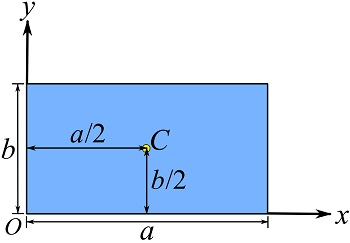
Find the centroid of a rectangular surface with the dimensions as shown.
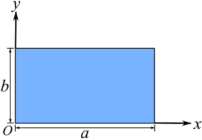
SOLUTION
Approach 1: double-integrals.
Consider a differential element as shown in the figure. As the sides of the element approaches zero in both directions,  and
and  . Therefore, we can write,
![\[\begin{split}\bar x&= \frac{\iint_A x dxdy}{\iint_A dxdy}=\frac{\int_0^a\int_0^b x dxdy}{\int_0^a\int_0^b dxdy}=\frac{\int_0^a x\left(\int_0^b dy \right)dx}{ab}=\frac{a^2b}{2ab}\\&=\frac{a}{2}\end{split}\]](https://engcourses-uofa.ca/wp-content/ql-cache/quicklatex.com-cb56dc08f49bd3d39679f69742dcc9df_l3.png "Rendered by QuickLaTeX.com")
And with a similar approach,
![\[\begin{split}\bar y&= \frac{\iint_A y dxdy}{\iint_A dxdy}\\&=\frac{b}{2}\end{split}\]](https://engcourses-uofa.ca/wp-content/ql-cache/quicklatex.com-17557339f950498e7003c1b667a04fd4_l3.png "Rendered by QuickLaTeX.com")
Note that  for the rectangular area.
Therefore the centroid or geometric center of a rectangle is located as shown,
Approach 2: single-variable integrals.
To express Eqs. 9.18 as single variable integrals, consider a differential element  as shown in the figure below and write the equation regarding
  .
.
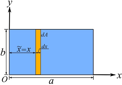
![\[\begin{split}\bar x&= \frac{\int_A \tilde x dA}{\int_A dA}=\frac{\int_0^a x bdx}{\int_0^a bdx}=\frac{a^2b}{2ab}\\&=\frac{a}{2}\end{split}\]](https://engcourses-uofa.ca/wp-content/ql-cache/quicklatex.com-57b50da511cfa28f28524df47351a7a6_l3.png "Rendered by QuickLaTeX.com")
To find  , consider a differential element as
  as shown below and write the corresponding equation.
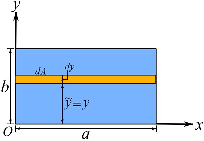
![\[\begin{split}\bar y&= \frac{\int_A \tilde y dA}{\int_A dA}=\frac{\int_0^b y ady}{\int_0^b ady}=\frac{b^2a}{2ab}\\&=\frac{b}{2}\end{split}\]](https://engcourses-uofa.ca/wp-content/ql-cache/quicklatex.com-412a1d212560ec70942922ff28992838_l3.png "Rendered by QuickLaTeX.com")
The same results are obtained using different differential elements.
We can use our knowledge on the centroid of a rectangular surface or area (see the previous example) to find the centroid of other flat surfaces. The following example demonstrates how to determine the centroid of a right-angle triangle.
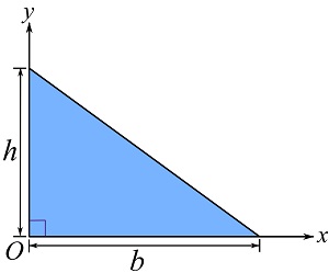
EXAMPLE 9.3.4
Determine the centroid of a right-angle triangular surface as shown.
SOLUTION
Consider a rectangular differential element  as shown. Based on our knowledge on the centroid of a rectangle, we know the centroid of the differential element as demonstrated in the figure. The term
  is the centroid of the differential element.
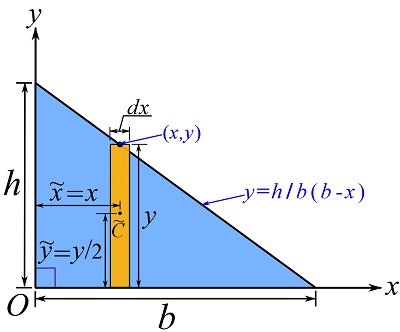
Therefore,
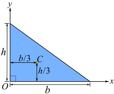
![\[\begin{split}\bar x&= \frac{\int_A \tilde x dA}{\int_A dA}=\frac{\int_0^b x ydx}{\int_0^b ydx}=\frac{\int_0^b \frac{h}{b}(b-x)x dx}{\int_0^b \frac{h}{b}(b-x)dx}\\&=\frac{b}{3}\end{split}\]](https://engcourses-uofa.ca/wp-content/ql-cache/quicklatex.com-b4633fafee38907215518da513ac9961_l3.png "Rendered by QuickLaTeX.com")
and,
![\[\begin{split}\bar y&= \frac{\int_A \tilde y dA}{\int_A dA}=\frac{\int_0^b \frac{y}{2}ydx}{\int_0^b ydx}=\frac{\int_0^b \frac{1}{2}\left(\frac{h}{b}(b-x)\right)^2 dx}{\int_0^b \frac{h}{b}(b-x)dx}\\&=\frac{h}{3}\end{split}\]](https://engcourses-uofa.ca/wp-content/ql-cache/quicklatex.com-9e0e1b8914cc462c69a241e75b407d5c_l3.png "Rendered by QuickLaTeX.com")
being shown as,
Remark: since we are integrating in the x direction (with dx as the integral variable), we need to express all other variables (e.g., y in this case) in terms of x.
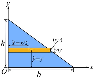
The above results can be also obtained using a differential element  as shown in the following figure. Try to solve the example using this element.
A rectangular differential element as used in the above example is also called a (differential) strip. The integrations for many problems can be simplified to single-variable integrals using strip elements. Figure 9.9 shows possible choices of strip elements for general cases where the area is defined by the region under a function  .
.

If an area is defined by the region confined between two functions as shown in Fig. 9.10, rectangular elements with varying heights between the two functions can be used.
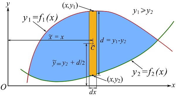
Figure 9.11 demonstrates the locations of the centroids of some typical flat (planar) surfaces.
Two applications
1- Thin volumes as differential elements. Knowing the centroid of a surface we can use thin slices as differential elements with known centroids to determine the centroid of a volume (e.g. Example 9.3.2). The following example further demonstrate this approach.
EXAMPLE 9.3.5
Determine the centroid of a half cone as shown. The radius  and the length
  of the half cone are known.

SOLUTION
Slicing the half cone with planes parallel to the x-z plane, we can have slices in the shape of a semi-circular area. Thereby, we can use this differential element for the integration.
As the element is thin along the y axis, its differential thickness is expressed as . The radius (or height) and width of the element are denoted by  and
and  , respectively with
  and
and 
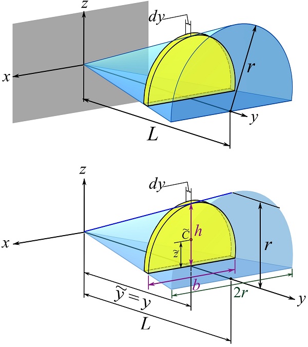
Therefore, the volume of the differential element is,
![\[ dV = \frac{1}{2}\pi h^2 dy =\frac{1}{2}\pi [(r/L)y]^2 dy \]](https://engcourses-uofa.ca/wp-content/ql-cache/quicklatex.com-58c15bb86dd9b83c0cfce48f93f4a7d8_l3.png "Rendered by QuickLaTeX.com")
Based on the coordinate system chosen and the centroid of a semi-circular area shown in Fig. 9.11, the coordinates of the centroid of the differential element are,
![\[\tilde x = 0\quad \tilde y = y \quad \tilde z = \frac{4h}{3\pi}\]](https://engcourses-uofa.ca/wp-content/ql-cache/quicklatex.com-f90f45e45e19fa7cd0e7144b89f853a4_l3.png "Rendered by QuickLaTeX.com")
With the above set up, we can calculate the integrals in Eqs. 9.14 as single-variable integrals.
For ,
![\[\begin{split}\bar x&= \frac{\int_V \tilde x dV}{\int_V dV} = \frac{\int_V 0 dV}{\int_V dV}\\&=0\end{split}\]](https://engcourses-uofa.ca/wp-content/ql-cache/quicklatex.com-0af85a76ccc792cdba46bb0b5befd9f1_l3.png "Rendered by QuickLaTeX.com")
For ,
![\[\bar y= \frac{\int_V \tilde y dV}{\int_V dV} = \frac{\int_0^L y (\frac{1}{2}\pi h^2) dy}{\int_0^L (\frac{1}{2}\pi h^2) dy}\]](https://engcourses-uofa.ca/wp-content/ql-cache/quicklatex.com-654663884c9e176ee17991eeb335700a_l3.png "Rendered by QuickLaTeX.com")
Substituting  , we get,
![\[\bar y = \frac{3L}{4}\]](https://engcourses-uofa.ca/wp-content/ql-cache/quicklatex.com-985c711477dbfe39204289767fec1512_l3.png "Rendered by QuickLaTeX.com")
For ,
![\[\bar z= \frac{\int_V \tilde z dV}{\int_V dV} = \frac{\int_0^L \frac{4h}{3\pi} (\frac{1}{2}\pi h^2) dy}{\int_0^L (\frac{1}{2}\pi h^2) dy}\]](https://engcourses-uofa.ca/wp-content/ql-cache/quicklatex.com-6d178d719af7b912593020d3c1ae2c5f_l3.png "Rendered by QuickLaTeX.com")
where substituting for leads to,
![\[\bar z = \frac{r}{\pi}\]](https://engcourses-uofa.ca/wp-content/ql-cache/quicklatex.com-d09e838f1915c621b3b060d652843ec7_l3.png "Rendered by QuickLaTeX.com")
In summary, we have  as already shown in Fig. 9.6.
2- Simplification of distributed loads. In section 3.5.2, it has been proved that a distributed load  along the x axis (Fig. 9.12) can be simplified as a single resultant force, with a magnitude of
  , and its line of action crossing a point on the the x axis.
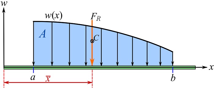
The terms and have been determined as,
![\[\begin{split}dF &= w(x)dx \ \text{ and }\ dM=xdF\\M_O&=\int_a^b dM\\F_R&=\int_a^bdF=\int_a^b w(x) dx\\\bar x &=\frac{M_O}{F_R}=\frac{\int_a^b x w(x) dx}{\int_a^b w(x) dx}\end{split}\]](https://engcourses-uofa.ca/wp-content/ql-cache/quicklatex.com-cc715903aa4d97e54f0ae676e6985597_l3.png "Rendered by QuickLaTeX.com")
which take the following geometric interpretations,
![\[\begin{split}dF &= dA\\dM&=x dA\end{split}\]](https://engcourses-uofa.ca/wp-content/ql-cache/quicklatex.com-4fa7114e2a2446650ae54f5b082b11ee_l3.png "Rendered by QuickLaTeX.com")
where id the differential element, i.e. a strip under the  curve.
![\[\begin{split}F_R &= \int_A dA = A\\\bar x &= \frac{\int_A x dA}{A}\end{split}\]](https://engcourses-uofa.ca/wp-content/ql-cache/quicklatex.com-0d6dc3fb1afdd38bcca824cac0e8589a_l3.png "Rendered by QuickLaTeX.com")
where  is the area of the region under and is the x coordinate of the centroid of the area (Fig. 9.12). Calculating and pertaining
  is an instant of the case shown in Fig. 9.9a or b.
Centroid of a line
The Centroid of a line (straight or curvy) in space (Fig. 9.13a) has the following coordinates
(9.19) ![\[\begin{split}\bar x&= \frac{\int_L \tilde x dL}{\int_L dL}\\\bar y&= \frac{\int_L \tilde y dL}{\int_L dL}\\\bar z&= \frac{\int_L \tilde z dL}{\int_L dL} \end{split}\]](https://engcourses-uofa.ca/wp-content/ql-cache/quicklatex.com-938cee656296201a0d204f1fe06b0631_l3.png "Rendered by QuickLaTeX.com")
where  are the coordinates of the centroid of a differential line element with a length of
  (Fig 9.13a). When the length of a differential line element is infinitesimal (approaching zero), the centroid of the element is actually at the location of the element. Therefore, ,
  , and
, and  for this element. The term
  equals the total length, , of the line.
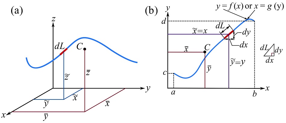
As shown in Fig. 9.13b, if a line (curve) is in a plane, say the x-y plane, the line can be expressed as a function,
![\[y=f(x) \quad \text {for } a\le x \le b \]](https://engcourses-uofa.ca/wp-content/ql-cache/quicklatex.com-9390b58e2d320679cde9ee8ee96a414f_l3.png "Rendered by QuickLaTeX.com")
or,
![\[x=g(y) \quad \text {for } c\le y \le d \]](https://engcourses-uofa.ca/wp-content/ql-cache/quicklatex.com-a43fbda993304eae0469f31f44ff6e79_l3.png "Rendered by QuickLaTeX.com")
By the Pythagoras’s theorem, the length of the differential element (Fig. 9.13b) is,
![\[dL=\sqrt{(dx)^2+(dy)^2}\]](https://engcourses-uofa.ca/wp-content/ql-cache/quicklatex.com-335b2a25d5098f490d17ebf42a9e5b66_l3.png "Rendered by QuickLaTeX.com")
Then, can be expressed in terms of  as
as  , or in terms of as
  , depending on the integration needs. See the following example for further explanation.
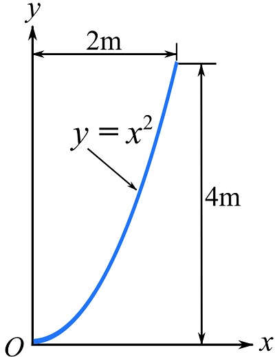
EXAMPLE 9.3.6
Find the centroid of a piece of a line having the shape of a parabolic arc as shown. This line can represent the center line of a rod bent into the shape of the arc.
SOLUTION
Set a Cartesian coordinate system and a differential element at an arbitrary point.
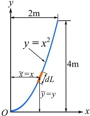
With  , we can write,
![\[dL=\sqrt{(dx)^2+(dy)^2}=\left (\sqrt{1+(\frac{dy}{dx})^2}\right )dx=\left (\sqrt{1+(2x)^2}\right )dx=\left (\sqrt{1+4x^2}\right )dx\]](https://engcourses-uofa.ca/wp-content/ql-cache/quicklatex.com-6a19c483b97cdb05f39b509f95a8d042_l3.png "Rendered by QuickLaTeX.com")
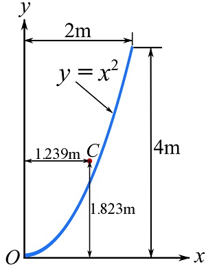
Therefore (using Eqs. 9.19),
![\[\begin{split}\bar x&= \frac{\int_L x dL}{\int_L dL}= \frac{\int_0^2 x \left (\sqrt{1+4x^2}\right )dx}{\int_0^2 \left (\sqrt{1+4x^2}\right )dx}=\frac{5.758}{4.647}\\&= 1.239\text{ m}\end{split}\]](https://engcourses-uofa.ca/wp-content/ql-cache/quicklatex.com-c844bd8b85900a018f05305cea017327_l3.png "Rendered by QuickLaTeX.com")
and,
![\[\begin{split}\bar y&= \frac{\int_L y dL}{\int_L dL}= \frac{\int_0^2 (x^2) \left (\sqrt{1+4x^2}\right )dx}{\int_0^2 \left (\sqrt{1+4x^2}\right )dx}=\frac{8.471}{4.647}\\&= 1.823 \text{ m}\end{split}\]](https://engcourses-uofa.ca/wp-content/ql-cache/quicklatex.com-207fe29f89e85e0f2fb49ee16a40d4de_l3.png "Rendered by QuickLaTeX.com")
which are shown as,
In some cases, integrating over x or y will complicate the calculation of the integrals. Other integral variables can be used to simplify the integration. The following example demonstrates the latter approach for finding the centroid of a circular arc.
EXAMPLE 9.3.7
Determine the centroid of a circular arc with a central angle of  and radius as shown.
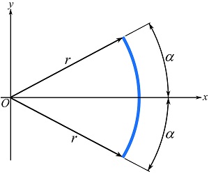
SOLUTION
Considering the center of the arc as the origin (figure below), the coordinates of points of the arc can be calculated as follows:
![\[ x= r\cos\theta\quad,\quad y=r\sin\theta\]](https://engcourses-uofa.ca/wp-content/ql-cache/quicklatex.com-3bca13f3480c4262c32b7bd7d766a8a6_l3.png "Rendered by QuickLaTeX.com")
The differential length, , of the arc as shown below is located by  . As is associated with an infinitesimal angle
  , it can be calculated as
  .
.
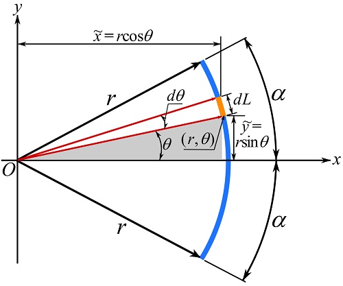
Expressing  and
and  of the differential element in terms of ,
![\[\tilde x = x =r\cos\theta\quad,\quad \tilde y = y = r\sin\theta\]](https://engcourses-uofa.ca/wp-content/ql-cache/quicklatex.com-579127baec434732771ad3d1264052ec_l3.png "Rendered by QuickLaTeX.com")
we can write,
![\[\begin{split}\bar x&= \frac{\int_L x dL}{\int_L dL}=\frac{\int_{-\alpha}^\alpha (r\cos\theta) rd\theta}{\int_{-\alpha}^\alpha rd\theta}\\&=\frac{r\sin\alpha}{\alpha}\end{split}\]](https://engcourses-uofa.ca/wp-content/ql-cache/quicklatex.com-e9567c32e7c2c3dfd397d12891375f4d_l3.png "Rendered by QuickLaTeX.com")
and,
![\[\begin{split}\bar y&= \frac{\int_L y dL}{\int_L dL}=\frac{\int_{-\alpha}^\alpha (r\sin\theta) rd\theta}{\int_{-\alpha}^\alpha rd\theta}\\&= 0\end{split}\]](https://engcourses-uofa.ca/wp-content/ql-cache/quicklatex.com-c258e9eb7825a7b7951283f50aeaf473_l3.png "Rendered by QuickLaTeX.com")
which are shown as,
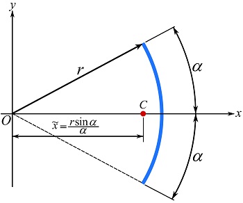
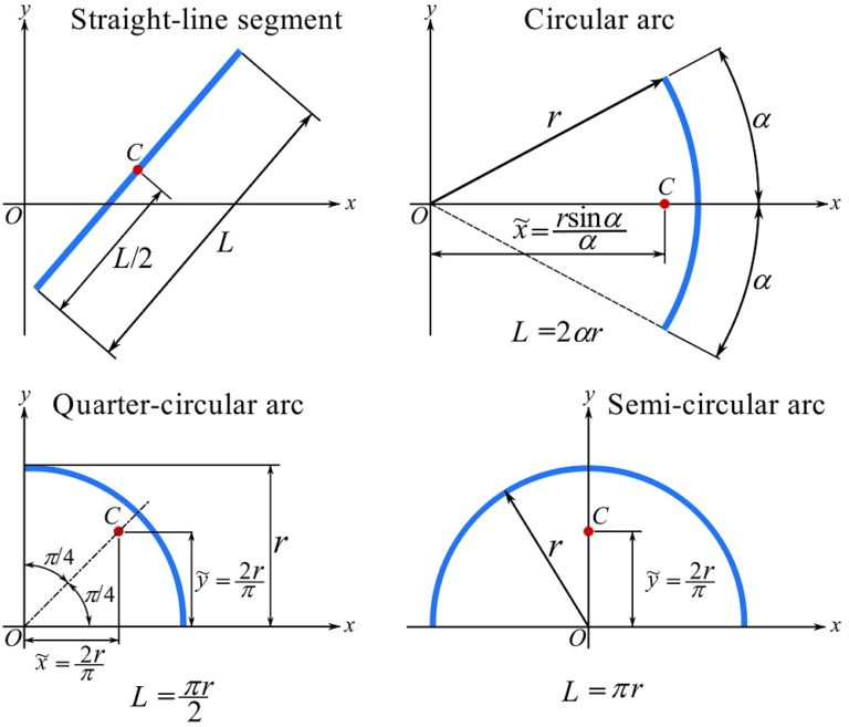
The centroid of some lines are shown in Fig 9.14.
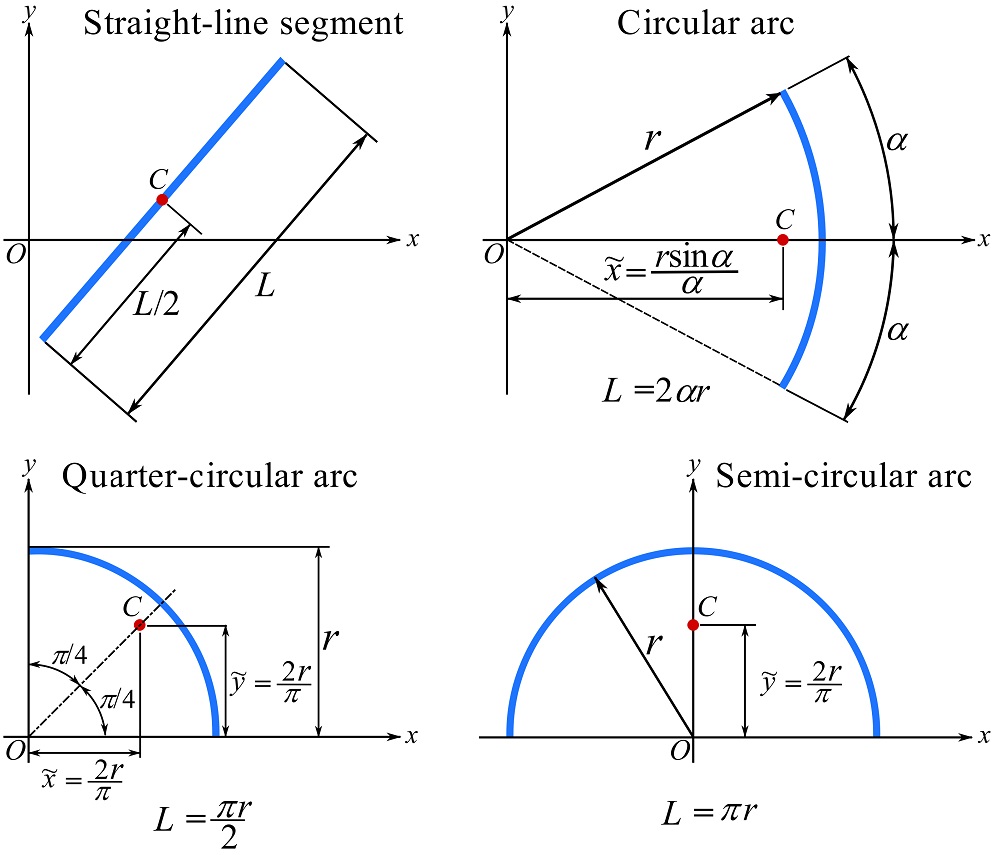
Remark: for finding the centroid of a slender body with a non-varying cross section following a line, its shape can be approximated by the center line of the body. For example, the shape of a piece of straight or curved rod, the dimensions of its cross section are much smaller than its length, can be approximated by its center line
Composite bodies
In the context of calculating the centroid, a composite body (a volume, surface, or line, continuous or not) is composed of several sub-bodies. For example, a rectangular surface can be partitioned into four triangular surfaces, or two rectangular surfaces. The boundaries specifying sub-bodies can be explicitly defined by regular or arbitrary shapes.
The centroid of a composite body becomes the sum of the integrations over all the sub-bodies. For a volume,  , composed of
  sub-volumes
  , Eqs. 9.14 become,
![\[\begin{split}\bar x&= \frac{\sum_{i=1}^n\int_{V_i} \tilde x dV}{\sum_1^n\int_{V_i} dV}\\\bar y&= \frac{\sum_{i=1}^n\int_{V_i} \tilde y dV}{\sum_1^n\int_{V_i} dV}\\\bar z&= \frac{\sum_{i=1}^n\int_{V_i} \tilde z dV}{\sum_1^n\int_{V_i} dV}\end{split}\]](https://engcourses-uofa.ca/wp-content/ql-cache/quicklatex.com-88bf7d101a4715d71f5da7fea40995d8_l3.png "Rendered by QuickLaTeX.com")
which can be written as,
(9.20) ![\[\begin{split}\bar x&= \frac{\sum \tilde x_i V_i}{\sum V_i}\\\bar y&= \frac{\sum \tilde y_i V_i}{\sum V_i}\\\bar z&= \frac{\sum \tilde z_i V_i}{\sum V_i}\end{split}\]](https://engcourses-uofa.ca/wp-content/ql-cache/quicklatex.com-4c932fb68668343b70af264127dee95f_l3.png "Rendered by QuickLaTeX.com")
where  , and
, and  denotes the coordinates of the centroid of the sub-volume
  .
.
For a (planar) surface, , composed of sub-surfaces  , Eqs. 9.18 become,
(9.21) ![\[\begin{split}\bar x&= \frac{\sum \tilde x_i A_i}{\sum A_i}\\\bar y&= \frac{\sum \tilde y_i A_i}{\sum A_i}\end{split}\]](https://engcourses-uofa.ca/wp-content/ql-cache/quicklatex.com-0080cefff04de33a861e1533c253383f_l3.png "Rendered by QuickLaTeX.com")
where  , and denotes the coordinates of the centroid of the sub-surface
  .
.
Lines can also be composed from sub-lines; therefore, Eqs. 9.19 take the following form for a (planar) line composed of sub-lines  ,
,
(9.22) ![\[\begin{split}\bar x&= \frac{\sum \tilde x_i L_i}{\sum L_i}\\\bar y&= \frac{\sum \tilde y_i L_i}{\sum L_i}\end{split}\]](https://engcourses-uofa.ca/wp-content/ql-cache/quicklatex.com-8266c32f5929bb874e04363773a559a4_l3.png "Rendered by QuickLaTeX.com")
where  , and denotes the coordinates of the centroid of the sub-line
  .
.
EXAMPLE 9.3.8
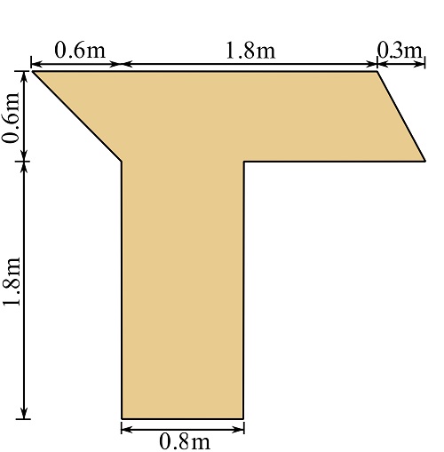
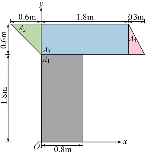
Determine the centoid of a planar surface with the dimensions shown.
SOLUTION
The surface can be partitioned into sub-surfaces as follows.
Set a Cartesian coordinate system and located the centroid of each surface with respect to itself. You can use the formulas in Fig. 9.11. The centroid of each shape is shown below.
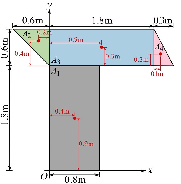
Use Eqs. 9.22 to calculate the centroid of the whole surface. Note that you need to express the coordinates of the centroid of each sub-surface with respect to the origin of the coordinate system.
The areas are calculated as,
![\[A_1 = 1.44 \text{m}^2,\quad A_2=0.18 \text{m}^2, \quad A_3=1.08 \text{m}^2,\quad A_4=0.09 \text{ m}^2\]](https://engcourses-uofa.ca/wp-content/ql-cache/quicklatex.com-9aabe846676605f693daa323cac04011_l3.png "Rendered by QuickLaTeX.com")
Therefore,
![\[\begin{split}\bar x&=\frac{\sum_1^4 \tilde x_i A_i}{\sum_1^4 A_i}=\frac{(0.4)(1.44)+(-0.2)(0.18)+(0.9)(1.08)+(1.8+0.1)(0.09)}{1.44+0.18+1.08+0.09}=\frac{1.683}{2.79}\\&=0.603\text{ m}\end{split}\]](https://engcourses-uofa.ca/wp-content/ql-cache/quicklatex.com-a979c441c243ec6593cb5b9de6cb80bc_l3.png "Rendered by QuickLaTeX.com")
and,
![\[\begin{split}\bar y&=\frac{\sum_1^4 \tilde y_i A_i}{\sum_1^4 A_i}=\frac{(0.9)(1.44)+(1.8+0.4)(0.18) +(1.8+0.3)(1.08)+(1.8+0.2)(0.09)}{1.44+0.18+1.08+0.09}\\&=\frac{4.14}{2.79}=1.484\text{ m}\end{split}\]](https://engcourses-uofa.ca/wp-content/ql-cache/quicklatex.com-677472c897b1b1125c7330be1ef47993_l3.png "Rendered by QuickLaTeX.com")
The centroid is located on the surface as,

Remark: It is convenience if we arrange the above calculations in a table as follows.
| sub-surface |  |  |  |  |  |
 | 0.4 | 0.9 | 1.44 | 0.576 | 1.296 |
 | -0.2 | 1.8+0.4=2.2 | 0.18 | -0.036 | 0.396 |
 | 0.9 | 1.8+0.3=2.1 | 1.08 | 0.972 | 2.268 |
 | 1.8+0.1=1.9 | 1.8+0.2+2.0 | 0.09 | 0.171 | 0.18 |
 |  |  |
Therefore,
![\[\bar x = \frac{\sum_1^4\tilde x_i A_i}{\sum_1^4 A_i}=0.603\text{ m}\]](https://engcourses-uofa.ca/wp-content/ql-cache/quicklatex.com-22c20008e8aff65e05683007f6847c65_l3.png "Rendered by QuickLaTeX.com")
![\[\bar y = \frac{\sum_1^4\tilde y_i A_i}{\sum_1^4 A_i}=1.484\text{ m}\]](https://engcourses-uofa.ca/wp-content/ql-cache/quicklatex.com-a7abccc010f479153f16d493c1c29fe1_l3.png "Rendered by QuickLaTeX.com")
Remark: partitioning an area into simpler sub-surfaces with known coordinates of centroids (from tables like Fig. 9.11) facilitates the calculations.
Remark: pay attention the negative coordinate values of the centroids of the sub-bodies.
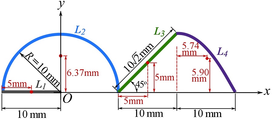
EXAMPLE 9.3.9
A bar is bent as shown in the figure. Determine its centroid with respect to the origin (O) of the coordinate system.
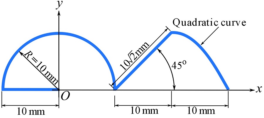
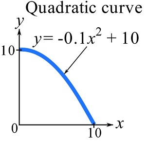
The segment of the bar in the shape of a quadratic curve is formulated as shown in the following figure.
SOLUTION
Consider the following sub-lines to locate the centroid of each sub-line.

For locating the centroids of the sub-lines  ,
,  and
and  , use the formulas in Fig. 9.14. To calculate the coordinates of the centroid of
  , we recruit Eq. 9.19 and write,
![\[\begin{split}\bar x&=\frac{\int_0^{10}x\left(\sqrt{1+(\frac{dy}{dx})^2}\right)dx}{\int_0^{10}\left(\sqrt{1+(\frac{dy}{dx})^2}\right)dx}=\frac{\int_0^{10}x\left(\sqrt{1+(-0.2x)^2}\right)dx}{\int_0^{10}\left(\sqrt{1+(-0.2x)^2}\right)dx}=\frac{84.84}{14.79}=5.74\text{ mm}\\\bar y&=\frac{\int_0^{10}y\left(\sqrt{1+(\frac{dy}{dx})^2}\right)dx}{\int_0^{10}\left(\sqrt{1+(\frac{dy}{dx})^2}\right)dx}=\frac{\int_0^{10}(-0.1x^2+10)\left(\sqrt{1+(-0.2x)^2}\right)dx}{\int_0^{10}\left(\sqrt{1+(-0.2x)^2}\right)dx}\\&=\frac{87.26}{14.79}=5.90\text{ mm}\end{split}\]](https://engcourses-uofa.ca/wp-content/ql-cache/quicklatex.com-f28c28b2ffd49f493c6c6fef9c5f3402_l3.png "Rendered by QuickLaTeX.com")
Note that the centroid of the quadratic curve is calculated with respect to the origin of its local coordinate system shown in Fig. 2.
The centroid of each sub-line with respect to a point of the sub-line is shown in the following figure.
Express the centoids with respect to point O, i.e. the origin of the coordinate system, and use Eqs. 9.22 to calculate the centroid of the whole line (bar). To facilitate the calculations, we use a table as follows.
| sub-line |  |  |  |  |  |
| -5.0 | 0.0 | 10.0 | -5.0 | 0 |
| 0.0 | 6.37 |  | 0 | 200.12 |
| 10+5=15 | 5.0 |  | 212.13 | 70.71 |
| 20+5.74=25.74 | 5.90 | 14.79 | 380.70 | 87.26 |
 |  |  |
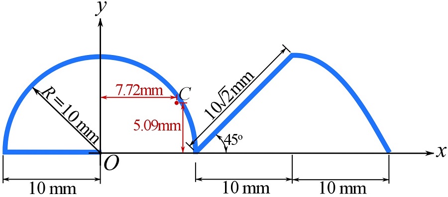
Therefore,
![\[\begin{split}\bar x&= \frac{\sum \tilde x_i L_i}{\sum L_i}= \frac{542.83}{70.35}=7.72\text{ mm}\\\bar y&= \frac{\sum \tilde y_i L_i}{\sum L_i}= \frac{542.83}{70.35}=5.09\text{ mm}\end{split}\]](https://engcourses-uofa.ca/wp-content/ql-cache/quicklatex.com-152c41e8c8c010d5c9c5f2a727577965_l3.png "Rendered by QuickLaTeX.com")
which are shown as,
Centroid of a body with empty parts
Some volumes, surfaces, or lines contain hollow or empty parts (regions); in other words, they can be regarded as a body with some subtracted or empty sub-bodies (Fig. 9.15). An empty part can be treated as a sub-body with negative volume, area, or length when calculating the centroid.
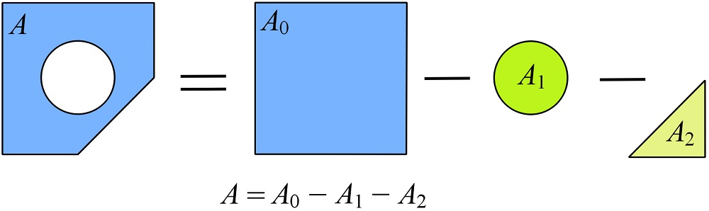
The following example clarifies how to treat empty parts when calculating the centroid.
EXAMPLE 9.3.10
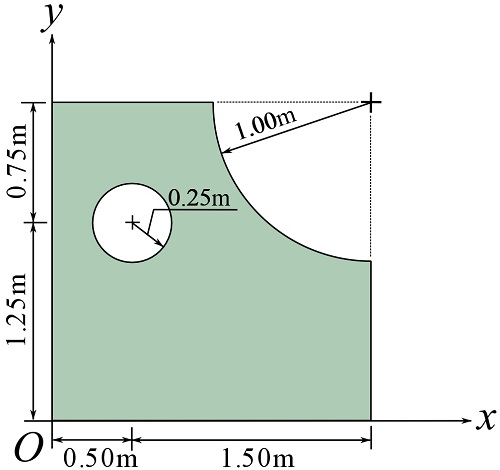
Locate the centroid of an area punched with a circular and a corner quarter-circular hole as shown.
SOLUTION
Use Eqs. 9.22 and subtract empty areas by assigning negative signs to their areas in the formulation (see Fig. 9.15).
Area of the intact rectangular area:  .
.
Area of the circular hole (empty):  .
.
Area of the quarter-circular hole (empty):  .
.
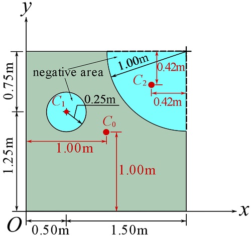
The locations of the centroids of the (intact) rectangular area ( ) and the empty areas (
 and
and  ) are shown below (use the formulas in Fig. 9.11).
Therefore,
![\[\begin{split}\bar x&= \frac{\sum \tilde x_i A_i}{\sum A_i}=\frac{(1)(4)+(0.5)(-0.2)+(2-0.42)(-0.79)}{4-0.2-0.79}\\&=0.88\text{ m}\end{split}\]](https://engcourses-uofa.ca/wp-content/ql-cache/quicklatex.com-918f4cc019c43c1c2b6558e8526d33ce_l3.png "Rendered by QuickLaTeX.com")
and,
![\[\begin{split}\bar y&= \frac{\sum \tilde x_i A_i}{\sum A_i}=\frac{(1)(4)+(1.25)(-0.2)+(2-0.42)(-0.79)}{4-0.2-0.79}\\&=0.83\text{ m}\end{split}\]](https://engcourses-uofa.ca/wp-content/ql-cache/quicklatex.com-769473dd20bf6079edc90f45effb4d73_l3.png "Rendered by QuickLaTeX.com")
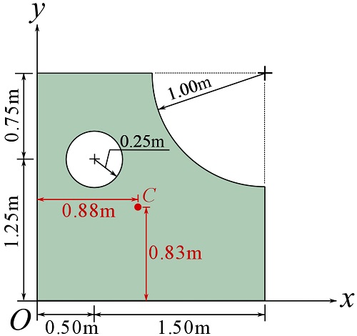
shown as,
To facilitate the calculations, we can use a table as follows.
| sub-surface | | | | | |
 | 1.0 | 1.0 | 4.0 | 4.0 | 4.0 |
| 0.5 | 1.25 | -0.20 | -0.1 | -0.25 |
| 2-0.42=1.58 | 2-0.42=1.58 | -0.79 | -1.25 | -1.25 |
 |  |  |
Therefore,
![\[\begin{split}\bar x&= \frac{2.65}{3.01}=0.88\text{ m}\\\bar y&= \frac{2.50}{3.01}=0.83\text{ m}\end{split}\]](https://engcourses-uofa.ca/wp-content/ql-cache/quicklatex.com-dcee8f689aea498784f1247f5d6b8244_l3.png "Rendered by QuickLaTeX.com")
Symmetry
A volume can have a plane(s) of symmetry that is a plane(s) dividing the body into two pieces that are mirror images of each other.
A planar body (area or line) can have a line(s) of symmetry that is a line(s) dividing the body into two pieces that are mirror images of each other.
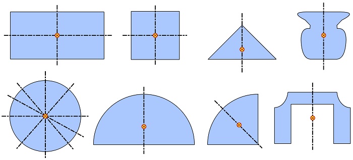
Symmetry is a property we can take advantage of when dealing with centroid problems. If a body has a plane(s) or line(s) of symmetry, then the centroid will lie on the plane(s) or line(s) of symmetry. Figure 9.16 shows examples of centroids being on the line(s) of symmetry of areas.
To prove the fact that the centroid of a symmetric body must lie on its line(s) of symmetry, consider an arbitrary planar surface and the y axis as the line of symmetry as shown in Fig 9.17.
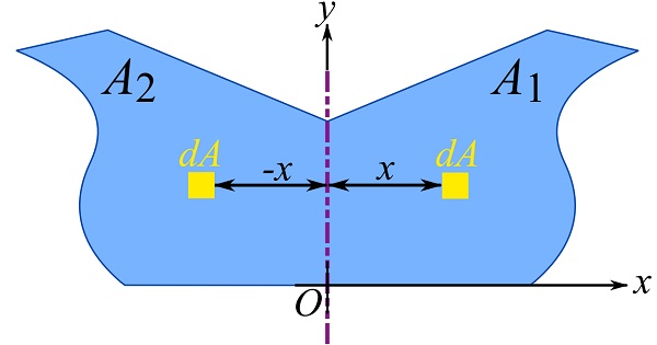
The line of symmetry partitions the area, , into two mirror areas and . Therefore,
![\[\bar x = \int_A xdA=\int_{A_1}xdA+\int_{A_2}xdA\]](https://engcourses-uofa.ca/wp-content/ql-cache/quicklatex.com-a5075d8048c474cb38982770ef53bdd3_l3.png "Rendered by QuickLaTeX.com")
Because the area is symmetric about the y axis, any differential area located at  in has a counterpart located at
  in . Therefore,
![\[\bar x = \int_A xdA=\int_{A_1}xdA+\int_{A_2}xdA=\int_{A_1}xdA+\int_{A_1}-xdA=\int_{A_1}(x-x)dA=0\]](https://engcourses-uofa.ca/wp-content/ql-cache/quicklatex.com-cd15a34faf040a8a799e30e15bac916c_l3.png "Rendered by QuickLaTeX.com")
meaning that the centroid must be on the line of symmetry, i.e the y axis.
Videos
Centroids (Continuous Body):
Centroids (Composite Body):