
Advanced Dynamics and Vibrations: Transfer matrices and periodic structures
Transfer Matrices – State Vectors for Vibrating Systems
For many MDOF systems, it is often more efficient to use a “shooting” technique rather than solve a boundary value problem. Essentially, we employ a series of initial value problems to find the solution to the boundary value problem. In vibrations, several numerical procedures have led to the “transfer matrix/state vector” approach. This includes the methods of Holzer and Myklestad’s for beams. This technique is an iterative technique where an estimate of the natural is used at one boundary then checked at the other and if not correct an iterative procedure is used to “hone-in-on” the answer (eg. Newton and Raphson). After the correct answer is found the mode is also known as the “states” have been calculated.
Transfer Matrices – State Vectors
In the transfer matrix approach, we follow the idea of the Holzer method and guess the eigenvalue (natural frequency). This approach can be extended to continuous systems.
We will introduce this for torsional and spring systems. We define the state of a position in the system as the force and displacement at that point.
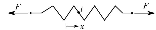
![\[ \{\mathfrak z\}_i = \begin{Bmatrix} x \\ F \end{Bmatrix}_i \text{ (axial)} \]](https://engcourses-uofa.ca/wp-content/ql-cache/quicklatex.com-7284500a5958db07cf64d58461d5711a_l3.png "Rendered by QuickLaTeX.com")
![\[ \{\mathfrak z\}_i = \begin{Bmatrix} \theta \\ T \end{Bmatrix}_i \text{ (torsional)} \]](https://engcourses-uofa.ca/wp-content/ql-cache/quicklatex.com-6cf4ac1b0fead9f2ea17d1a3c092f64f_l3.png "Rendered by QuickLaTeX.com")
Transfer Matrix – relates the state vectors at two points in the system
![\[ F_{i + 1} = F_i \]](https://engcourses-uofa.ca/wp-content/ql-cache/quicklatex.com-cc14b890d3e17e2418d40ef750816a61_l3.png "Rendered by QuickLaTeX.com")
![\[x_{i+1} = x_i + \frac{F_i}{k_i} \]](https://engcourses-uofa.ca/wp-content/ql-cache/quicklatex.com-6c50ae2369ea1796eb6a34db8376ecc4_l3.png "Rendered by QuickLaTeX.com")
Therefore:
![\[ \begin{split} \begin{Bmatrix} x \\ F \end{Bmatrix}_{i+1} &= \begin{bmatrix} 1 & \frac{1}{k_i} \\ 0 & 1 \end{bmatrix} \begin{Bmatrix} x \\ F \end{Bmatrix}_i \\&= [z] \{ \mathfrak z \}_i \end{split} \]](https://engcourses-uofa.ca/wp-content/ql-cache/quicklatex.com-db19333d108dcf334090ababbaa7a884_l3.png "Rendered by QuickLaTeX.com")
This is called a field transfer matrix.
If we have a discontinuity of mass at a point:
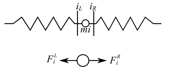
![\[ \begin{split} \sum F_x &= m_i \ddot{x}_i \\&= F_i^R - F_i^L \end{split} \]](https://engcourses-uofa.ca/wp-content/ql-cache/quicklatex.com-6c2e8db8c7315c5ee7c6e3eb7eb8e06c_l3.png "Rendered by QuickLaTeX.com")
![\[ x_i^L = x_i^R \]](https://engcourses-uofa.ca/wp-content/ql-cache/quicklatex.com-c2b7d7602fe1e5dcae88cdb92ccce6a5_l3.png "Rendered by QuickLaTeX.com")
Assume  (SHM). Therefore:
![\[ -m_ip^2x_i = F_i^R - F_i^L \]](https://engcourses-uofa.ca/wp-content/ql-cache/quicklatex.com-3943d24199116d9a85d9328b025af326_l3.png "Rendered by QuickLaTeX.com")
Therefore:
![\[ \begin{split} \begin{Bmatrix} x \\ F \end{Bmatrix}_i^R &= \begin{bmatrix} 1 & 0 \\ -m_ip^2 & 1 \end{bmatrix} \begin{Bmatrix} x \\ F \end{Bmatrix}_i^L \\&= [p] \{ \mathfrak z \}_i^L \end{split} \]](https://engcourses-uofa.ca/wp-content/ql-cache/quicklatex.com-193ed8390848d06b9926ef5a7b3ab35c_l3.png "Rendered by QuickLaTeX.com")
Where the point transfer matrix is ![[p]](https://engcourses-uofa.ca/wp-content/ql-cache/quicklatex.com-30d3134ad19b660aefddb8b07b4e63d7_l3.png "Rendered by QuickLaTeX.com") . We can combine these to generate a transfer matrix from one position to another which are at like locations.
. We can combine these to generate a transfer matrix from one position to another which are at like locations.
![\[ \begin{split} \{ \mathfrak z \}_{i+1}^R &= [p]_{i+1} \{ \mathfrak z \}_{i+1}^L \\&= [p]_{i+1} [z] \{ \mathfrak z \}_i^R \end{split} \]](https://engcourses-uofa.ca/wp-content/ql-cache/quicklatex.com-cdf434aea3ea9039fd0f8b2be41894ad_l3.png "Rendered by QuickLaTeX.com")
Therefore:
![\[ \begin{split} \{ \mathfrak z \}_{i+1}^R &= \begin{bmatrix} 1 & 0 \\ -m_ip & 1 \end{bmatrix} \begin{bmatrix} 1 & \frac{1}{k_i} \\ 0 & 1 \end{bmatrix} \{ \mathfrak z \}_i^R \\&= \begin{bmatrix} 1 & \frac{1}{k_i} \\ -p^2m_i & 1 - \frac{m_ip^2}{k_i} \end{bmatrix} \{ \mathfrak z \}_i^R \end{split} \]](https://engcourses-uofa.ca/wp-content/ql-cache/quicklatex.com-59431af65c2a92aee7dceffb1ca79e2a_l3.png "Rendered by QuickLaTeX.com")
Example 1

![\[ \{ \mathfrak z \}_1^L = [Z] \{\mathfrak z\}_o = \begin{bmatrix} 1 & \frac{1}{k} \\ 0 & 1 \end{bmatrix} \{ \mathfrak z \}_o \]](https://engcourses-uofa.ca/wp-content/ql-cache/quicklatex.com-f87cf462c2d535c74a8de87a9353de29_l3.png "Rendered by QuickLaTeX.com")
![\[ \begin{split} \{ \mathfrak z \}_1^R &= \begin{bmatrix} 1 & 0 \\ -mp^2 & 1 \end{bmatrix} \{ \mathfrak z \}_1^L \\&= \begin{bmatrix} 1 & 0 \\ -mp^2 & 1 \end{bmatrix} \begin{bmatrix} 1 & \frac{1}{k} \\ 0 & 1 \end{bmatrix} \begin{Bmatrix} 0 \\ F \end{Bmatrix}_o \end{split} \]](https://engcourses-uofa.ca/wp-content/ql-cache/quicklatex.com-ce127801fd8f331ca73c13415fcc56d4_l3.png "Rendered by QuickLaTeX.com")
![\[ \begin{Bmatrix} x \\ 0 \end{Bmatrix}_1^R = \begin{bmatrix} 1 & \frac{1}{k} \\ -mp^2 & 1 - \frac{mp^2}{k} \end{bmatrix} \begin{Bmatrix} 0 \\ F \end{Bmatrix}_o \]](https://engcourses-uofa.ca/wp-content/ql-cache/quicklatex.com-b11859e53bea84dadeaacd3d9e187038_l3.png "Rendered by QuickLaTeX.com")
![\[ 0 = \Big(1 - \frac{mp^2}{k} \Big) F_o \]](https://engcourses-uofa.ca/wp-content/ql-cache/quicklatex.com-18ddfcfc5237d9ae73a95ef7e2a3bd67_l3.png "Rendered by QuickLaTeX.com")
Therefore:
![\[ 1 - \frac{mp^2}{k} = 0 \]](https://engcourses-uofa.ca/wp-content/ql-cache/quicklatex.com-deaf9acccb3809a6c89ef3e22e9329a0_l3.png "Rendered by QuickLaTeX.com")
![\[ p^2 = \frac{k}{m} \]](https://engcourses-uofa.ca/wp-content/ql-cache/quicklatex.com-e3e7c7251fbfd603c58eeaf09e577b77_l3.png "Rendered by QuickLaTeX.com")
A long way to get this simple result.
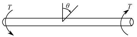
Consider a torsional system:
Then the positive directions are similar to the analogous linear case. The field equations are then:
![\[ \begin{Bmatrix} \theta \\ T \end{Bmatrix}_i = \begin{bmatrix} 1 & \frac{1}{\hat{k}_1} \\ 0 & 1 \end{bmatrix} \begin{Bmatrix} \theta \\ T \end{Bmatrix}_{i-1} \]](https://engcourses-uofa.ca/wp-content/ql-cache/quicklatex.com-2afc9faf862c96f2f1b4bb808cbcae70_l3.png "Rendered by QuickLaTeX.com")
The point matrix is:
![\[ \begin{Bmatrix} \theta \\ T \end{Bmatrix}_i^R = \begin{bmatrix} 1 & 0 \\ -J_ip^2 & 1 \end{bmatrix} \begin{Bmatrix} \theta \\ T \end{Bmatrix}_i^L \]](https://engcourses-uofa.ca/wp-content/ql-cache/quicklatex.com-03777c2fe2086dba567a0cd2d66cbad1_l3.png "Rendered by QuickLaTeX.com")
It is often useful to divide the torques by a  to make them non-dimesional as well.
![\[ \begin{Bmatrix} \theta \\ T \end{Bmatrix} = \begin{bmatrix} 1 & 0 \\ \frac{-J_ip^2}{\hat{k}} & 1 \end{bmatrix} \begin{Bmatrix} \theta \\ \tilde{T} \end{Bmatrix}_i \]](https://engcourses-uofa.ca/wp-content/ql-cache/quicklatex.com-441f3dfdf255d0ead4151634fb364e09_l3.png "Rendered by QuickLaTeX.com")
![\[ \begin{Bmatrix} \theta \\ T \end{Bmatrix} = \begin{bmatrix} 1 & \frac{\hat{k}}{\hat{k}_i} \\ 0 & 1 \end{bmatrix} \begin{Bmatrix} \theta \\ \tilde{T} \end{Bmatrix}_{i-1} \]](https://engcourses-uofa.ca/wp-content/ql-cache/quicklatex.com-933ea402edb3fe30941b6d9899b755c3_l3.png "Rendered by QuickLaTeX.com")
Example 2
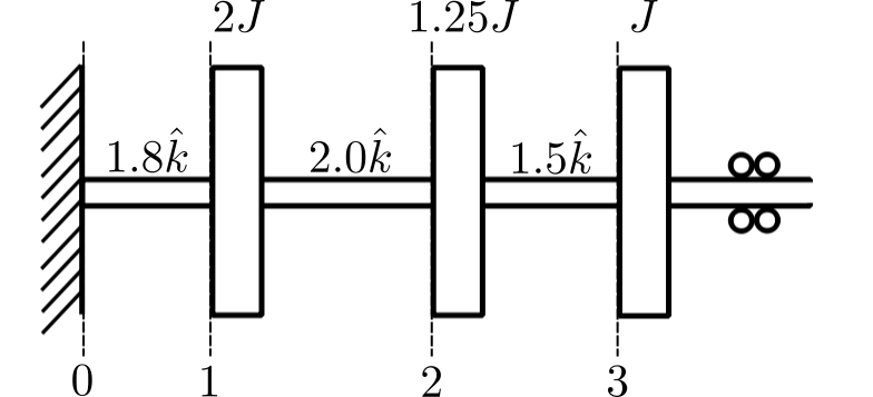
![\[ \hat{k} = 1 \cdot 10^6 \text{ lbs in/rad} \]](https://engcourses-uofa.ca/wp-content/ql-cache/quicklatex.com-e2cbb209e24951066400730dcff6d989_l3.png "Rendered by QuickLaTeX.com")
![\[ J = 100 \text{ lb in sec}^2 \]](https://engcourses-uofa.ca/wp-content/ql-cache/quicklatex.com-2e5fea1c665ef2edecabeb83a14269d5_l3.png "Rendered by QuickLaTeX.com")
![\[ \{ \mathfrak z \}_B^R = [p]_3 [z]_{2-3} [p]_2 [z]_{1-2} [p]_1 [z]_{0-1} \{ \mathfrak z \}_o \]](https://engcourses-uofa.ca/wp-content/ql-cache/quicklatex.com-98f421ef8b33968cce732d2658ae6508_l3.png "Rendered by QuickLaTeX.com")
![\[ \begin{Bmatrix} \theta \\ 0 \end{Bmatrix}_3^R = \begin{bmatrix} a_{11} & a_{12} \\ a_{21} & a_{22} \end{bmatrix} \begin{Bmatrix} 0 \\ T \end{Bmatrix}_o \]](https://engcourses-uofa.ca/wp-content/ql-cache/quicklatex.com-988cee63b0626f4f097d7f2ec02a03fa_l3.png "Rendered by QuickLaTeX.com")
Note that  and
and  are not required. It is sometimes better to non-dimensionalize the equations by dividing the torques by . Therefore:
![\[ \begin{bmatrix} 1 & \frac{1}{1.8} \\ 0 & 1 \end{bmatrix} = [z]_{0-1} \]](https://engcourses-uofa.ca/wp-content/ql-cache/quicklatex.com-6cd4b3f94e14bdef526b81d40cf31ae1_l3.png "Rendered by QuickLaTeX.com")
![\[ \begin{bmatrix} 1 & 0 \\ -\frac{p^2(2J)}{\hat{k}} & 1 \end{bmatrix} = [p]_1 \]](https://engcourses-uofa.ca/wp-content/ql-cache/quicklatex.com-736c51806bc0caf2a8321306c653e6be_l3.png "Rendered by QuickLaTeX.com")
Now we have only to choose the value of  . Assume:
![\[ \frac{p^2J}{\hat{k}} = 0.2 \]](https://engcourses-uofa.ca/wp-content/ql-cache/quicklatex.com-6a329508267b1f1ea15ed88d0a44580a_l3.png "Rendered by QuickLaTeX.com")
Then:
![\[ \begin{bmatrix} 0 \\ T \end{bmatrix}_o = \mathfrak z_o \]](https://engcourses-uofa.ca/wp-content/ql-cache/quicklatex.com-7533c38af0ef86c7a3b69e1efc16fe5f_l3.png "Rendered by QuickLaTeX.com")
![\[ \begin{bmatrix} 1 & 0.5556 \\ 0 & 1 \end{bmatrix} \begin{bmatrix} 0 \\ T \end{bmatrix}_o = \mathfrak z_1^L \]](https://engcourses-uofa.ca/wp-content/ql-cache/quicklatex.com-d6bd4e0fdd1adc1ac3c13d692c9d4a3d_l3.png "Rendered by QuickLaTeX.com")
![\[ \begin{bmatrix} 1 & 0.5556 \\ -0.4 & 0.7778 \end{bmatrix} \begin{bmatrix} 0 \\ T \end{bmatrix} = \begin{bmatrix} 1 & 0 \\ -0.4 & 1 \end{bmatrix} \begin{bmatrix} 1 & 0.5556 \\ 0 & 1 \end{bmatrix} \begin{bmatrix} 0 \\ T \end{bmatrix} = \mathfrak z_1^R \]](https://engcourses-uofa.ca/wp-content/ql-cache/quicklatex.com-2a97990f93d0389af76c4f5726d2935f_l3.png "Rendered by QuickLaTeX.com")
![\[ \begin{bmatrix} 0.8 & 0.9449 \\ -0.4 & 0.7778 \end{bmatrix} \begin{bmatrix} 0 \\ T \end{bmatrix} = \begin{bmatrix} 1 & 0.5 \\ 0 & 1 \end{bmatrix} \begin{bmatrix} 1 & 0.5556 \\ -0.4 & 0.7778 \end{bmatrix} \begin{bmatrix} 0 \\ T \end{bmatrix}_o = \mathfrak z_2^L \]](https://engcourses-uofa.ca/wp-content/ql-cache/quicklatex.com-5d697973ca5b8cfe07bd8f54e890a2b3_l3.png "Rendered by QuickLaTeX.com")
![\[ \begin{bmatrix} 0.8 & 0.9449 \\ -0.6 & 0.5416 \end{bmatrix} \begin{bmatrix} 0 \\ T \end{bmatrix} = \begin{bmatrix} 1 & 0 \\ -0.25 & 1 \end{bmatrix} \begin{bmatrix} 0.8 & 0.9449 \\ -0.4 & 0.7778 \end{bmatrix} \begin{bmatrix} 0 \\ T \end{bmatrix} = \mathfrak z_2^R \]](https://engcourses-uofa.ca/wp-content/ql-cache/quicklatex.com-72b88440532f514f778fb441485885ca_l3.png "Rendered by QuickLaTeX.com")
![\[ \begin{bmatrix} 0.4 & 1.3060 \\ -0.6 & 0.5416 \end{bmatrix} \begin{bmatrix} 0 \\ T \end{bmatrix}_o = \begin{bmatrix} 1 & 0.6667 \\ 0 & 1 \end{bmatrix} \begin{bmatrix} 0.8 & 0.9449 \\ -0.6 & 0.5416 \end{bmatrix} \begin{bmatrix} 0 \\ T \end{bmatrix}_o = \mathfrak z_3^L \]](https://engcourses-uofa.ca/wp-content/ql-cache/quicklatex.com-92e0432d8138c03bbadca66e3728003b_l3.png "Rendered by QuickLaTeX.com")
![\[ \begin{bmatrix} 0.4 & 1.3060 \\ -0.68 & 0.2804 \end{bmatrix} \begin{bmatrix} 0 \\ T \end{bmatrix}_o = \begin{bmatrix} 1 & 0 \\ -0.2 & 1 \end{bmatrix} \begin{bmatrix} 0.4 & 1.3060 \\ -0.6 & 0.5416 \end{bmatrix} \begin{bmatrix} 0 \\ T \end{bmatrix}_o = \mathfrak z_3^R \]](https://engcourses-uofa.ca/wp-content/ql-cache/quicklatex.com-7c62af46be4772823c7ecb5c3a567926_l3.png "Rendered by QuickLaTeX.com")
This is not a natural frequency as  and it should be zero. Also, look at the mode shape:
![\[ \begin{Bmatrix} \theta_1 \\ \theta_2 \\ \theta_3 \end{Bmatrix} = \begin{Bmatrix} 0.5556 \\ 0.9449 \\ 1.3060 \end{Bmatrix} \text{ (not correct)} \]](https://engcourses-uofa.ca/wp-content/ql-cache/quicklatex.com-a58f8f3da4e2a368fbb048896084e1d9_l3.png "Rendered by QuickLaTeX.com")
The correct answer is  .
.
Non Dimensionalized Matrices
![\[ \begin{bmatrix} 1 & \frac{1}{1.8} \\ 0 & 1 \end{bmatrix} = [z]_{0-1} \quad \begin{bmatrix} 1 & 0 \\ \frac{-p^2(2J)}{k} & 1 \end{bmatrix} = [p]_1 \]](https://engcourses-uofa.ca/wp-content/ql-cache/quicklatex.com-0c77738d57b459d641661b7da2b7696d_l3.png "Rendered by QuickLaTeX.com")
![\[ \begin{bmatrix} 1 & \frac{1}{2} \\ 0 & 1 \end{bmatrix} = [z]_{1-2} \quad \begin{bmatrix} 1 & 0 \\ \frac{-p^2(1.25J)}{k} & 1 \end{bmatrix} = [p]_2 \]](https://engcourses-uofa.ca/wp-content/ql-cache/quicklatex.com-70205bf8457e739542a7fdbf2e3dce81_l3.png "Rendered by QuickLaTeX.com")
![\[ \begin{bmatrix} 1 & \frac{1}{1.5} \\ 0 & 1 \end{bmatrix} = [z]_{2-3} \quad \begin{bmatrix} 1 & 0 \\ \frac{-p^2(J)}{k} & 1 \end{bmatrix} = [p]_3 \]](https://engcourses-uofa.ca/wp-content/ql-cache/quicklatex.com-a7b467d1d529716559b9fe2e6822e003_l3.png "Rendered by QuickLaTeX.com")
Assume  . Then:
![\[ \begin{bmatrix} 0 \\ \tilde{T} \end{bmatrix}_o = \{ \mathfrak z\}_o \]](https://engcourses-uofa.ca/wp-content/ql-cache/quicklatex.com-b5b7f8f1834a896c835e0e9351def213_l3.png "Rendered by QuickLaTeX.com")
![\[ \begin{bmatrix} 1 & 0.5556 \\ 0 & 1 \end{bmatrix} \begin{bmatrix} 0 \\ \tilde{T} \end{bmatrix}_o = \{ \mathfrak z \}_1^L \]](https://engcourses-uofa.ca/wp-content/ql-cache/quicklatex.com-bfe830c875c12a5317a67106209327d5_l3.png "Rendered by QuickLaTeX.com")
![\[ \begin{bmatrix} 1 & 0.5556 \\ -0.6 & 0.6666 \end{bmatrix} \begin{bmatrix} 0 \\ \tilde{T} \end{bmatrix}_o = \begin{bmatrix} 1 & 0 \\ -0.6 & 1 \end{bmatrix} \begin{bmatrix} 1 & 0.5556 \\ 0 & 1 \end{bmatrix} \begin{bmatrix} 0 \\ \tilde{T} \end{bmatrix}_o = \{ \mathfrak z \}_1^R \]](https://engcourses-uofa.ca/wp-content/ql-cache/quicklatex.com-25a373b1a465043da037e7c401a180f4_l3.png "Rendered by QuickLaTeX.com")
![\[ \begin{bmatrix} 0.7 & 0.8889 \\ -0.6 & 0.6666 \end{bmatrix} \begin{bmatrix} 0 \\ \tilde{T} \end{bmatrix}_o = \begin{bmatrix} 1 & 0.5 \\ 0 & 1 \end{bmatrix} \begin{bmatrix} 1 & 0.5556 \\ -0.6 & 0.6666 \end{bmatrix} \begin{bmatrix} 0 \\ \tilde{T} \end{bmatrix}_o = \{ \mathfrak z \}_2^L \]](https://engcourses-uofa.ca/wp-content/ql-cache/quicklatex.com-c984fd8c4b263ebe186029bd375737d2_l3.png "Rendered by QuickLaTeX.com")
![\[ \begin{bmatrix} 0.7 & 0.8889 \\ -0.8625 & 0.3333 \end{bmatrix} \begin{bmatrix} 0 \\ \tilde{T} \end{bmatrix} = \begin{bmatrix} 1 & 0 \\ -0.375 & 1 \end{bmatrix} \begin{bmatrix} 0.7 & 0.8889 \\ -0.6 & 0.6666 \end{bmatrix} \begin{bmatrix} 0 \\ \tilde{T} \end{bmatrix} = \{ \mathfrak z \}_2^R \]](https://engcourses-uofa.ca/wp-content/ql-cache/quicklatex.com-b807ef8fc771a38849c61f47b5718d04_l3.png "Rendered by QuickLaTeX.com")
![\[ \begin{bmatrix} 0.1250 & 1.10511 \\ -0.8625 & 0.3333 \end{bmatrix} \begin{bmatrix} 0 \\ \tilde{T} \end{bmatrix} = \begin{bmatrix} 1 & 0.6667 \\ 0 & 1 \end{bmatrix} \begin{bmatrix} 0.7 & 0.8829 \\ -0.8625 & 0.3333 \end{bmatrix} \begin{bmatrix} 0 \\ \tilde{T} \end{bmatrix} = \{ \mathfrak z \}_3^L \]](https://engcourses-uofa.ca/wp-content/ql-cache/quicklatex.com-8f26558d29ca2a4bde1ca2c78dfbbba2_l3.png "Rendered by QuickLaTeX.com")
![\[ \begin{bmatrix} 0.1250 & 1.10511 \\ 0.9000 & 0.0177 \end{bmatrix} \begin{bmatrix} 0 \\ \tilde{T} \end{bmatrix} = \begin{bmatrix} 1 & 0 \\ -0.3 & 1 \end{bmatrix} \begin{bmatrix} 0.1250 & 1.10511 \\ -0.8625 & 0.3333 \end{bmatrix} \begin{bmatrix} 0 \\ T \end{bmatrix} = \{ \mathfrak z \}_3^R \]](https://engcourses-uofa.ca/wp-content/ql-cache/quicklatex.com-f1e5404e082c09ab32a92ec52e1628e4_l3.png "Rendered by QuickLaTeX.com")
Therefore, close at  . Modal vector is:
![\[ \begin{Bmatrix} 0.5556 \\ 0.8889 \\ 1.1051 \end{Bmatrix} = \begin{Bmatrix} \theta_1 \\ \theta_2 \\ \theta_3 \end{Bmatrix} \]](https://engcourses-uofa.ca/wp-content/ql-cache/quicklatex.com-684f14b0ec0ca6760dce8cb33c2d64c9_l3.png "Rendered by QuickLaTeX.com")
Where to start, use Dunkerley’s technique.
![\[ \frac{1}{p_1^2} < \frac{1}{p_{11}^2} + \frac{1}{p_{22}^2} + \frac{1}{p_{33}^2} \]](https://engcourses-uofa.ca/wp-content/ql-cache/quicklatex.com-63e35b9d7d10de72f45171e690961aad_l3.png "Rendered by QuickLaTeX.com")
![\[ p_{11}^2 = \frac{1.8}{2} \frac{k}{J} \]](https://engcourses-uofa.ca/wp-content/ql-cache/quicklatex.com-afce8af6033fa97debdba4aaccedf488_l3.png "Rendered by QuickLaTeX.com")
![\[ p_{22}^2 = \frac{\frac{1}{\frac{1}{1.8} + \frac{1}{2.0}}}{1.25} \frac{k}{J} \]](https://engcourses-uofa.ca/wp-content/ql-cache/quicklatex.com-d191fd2d25e32f8ca101c2569fe0f978_l3.png "Rendered by QuickLaTeX.com")
![\[ p_{33}^2 = \frac{\frac{1}{\frac{1}{1.8} + \frac{1}{2.0} + \frac{1}{1.5}}}{1} \frac{k}{J}\]](https://engcourses-uofa.ca/wp-content/ql-cache/quicklatex.com-31cf7847d758a9808e0ac875bbd8478a_l3.png "Rendered by QuickLaTeX.com")
Therefore:
![\[ p_{11}^2 = 0.9 \frac{k}{J} \]](https://engcourses-uofa.ca/wp-content/ql-cache/quicklatex.com-e1db15aff53599011e2b62bcdfda99d3_l3.png "Rendered by QuickLaTeX.com")
![\[ p_{22}^2 = 0.758 \frac{k}{J} \]](https://engcourses-uofa.ca/wp-content/ql-cache/quicklatex.com-01601de96666cba0c419958763d4b77c_l3.png "Rendered by QuickLaTeX.com")
![\[ p_{33}^2 = 0.581 \frac{k}{J} \]](https://engcourses-uofa.ca/wp-content/ql-cache/quicklatex.com-5335fd5ea2bf0337908ecb21c4ecbc2f_l3.png "Rendered by QuickLaTeX.com")
Therefore:
![\[ \frac{1}{p_1^2} < \Big( \frac{1}{0.9} + \frac{1}{0.758} + \frac{1}{0.581} \Big) \frac{J}{k} \]](https://engcourses-uofa.ca/wp-content/ql-cache/quicklatex.com-8911e8f28b7e5efacffc7e611ea799da_l3.png "Rendered by QuickLaTeX.com")
Therefore:
![\[ p_1^2 > 0.241 \frac{k}{J} \]](https://engcourses-uofa.ca/wp-content/ql-cache/quicklatex.com-03e431abfd6dcaba4bbce98549238906_l3.png "Rendered by QuickLaTeX.com")
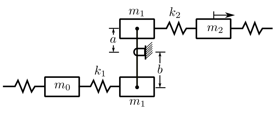
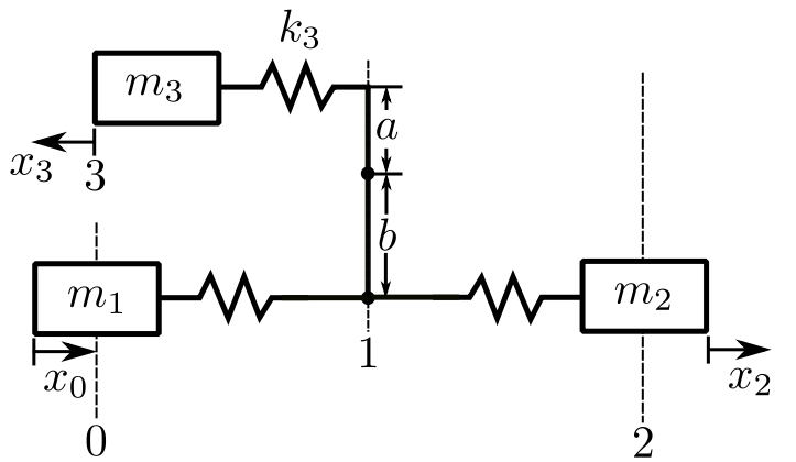
Release Point
Consider that there are masses at the ends of the lever  .
.
Again, we wish to go from  to
to  .
.
![\[ x_1^R = -\frac{a}{b}x_1^L \]](https://engcourses-uofa.ca/wp-content/ql-cache/quicklatex.com-3bbf7192f75b3785fa560d965bf9effc_l3.png "Rendered by QuickLaTeX.com")
![\[ \alpha = \frac{a}{b} \]](https://engcourses-uofa.ca/wp-content/ql-cache/quicklatex.com-7400e03cfa5fc01442bdc37cbf33a2ed_l3.png "Rendered by QuickLaTeX.com")
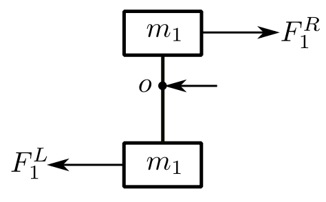
![\[ \begin{split} +\circlearrowleft \sum M_o &= (m_1b^2 + m_1^1a^2) \frac{\ddot{x}_1^L} {b} \\&= -F_1^R(a) - F_1^L(b) \end{split} \]](https://engcourses-uofa.ca/wp-content/ql-cache/quicklatex.com-448dbc21d4f08f630dca08895463f4f7_l3.png "Rendered by QuickLaTeX.com")
![\[ \begin{split} F_1^R &= -F_1^L \frac{b}{a} + (m_1b^2 + m_1^1a^2) \frac{p^2x_1^L}{ab} \\&= -\frac{F_1^L}{\alpha} + \Big(\frac{m_1}{\alpha} + m_1^1\alpha \Big) p^2x_1^L \end{split} \]](https://engcourses-uofa.ca/wp-content/ql-cache/quicklatex.com-7545f77508261cb2d80878d46d3ba63b_l3.png "Rendered by QuickLaTeX.com")
Therefore:
![\[ \begin{Bmatrix} x \\ F \end{Bmatrix}_1^R = \begin{bmatrix} -\alpha & 0 \\ p^2 (\frac{m_1}{\alpha} + m_1^1\alpha) & -\frac{1}{\alpha} \end{bmatrix} \begin{Bmatrix} x \\ F \end{Bmatrix}_1^L \]](https://engcourses-uofa.ca/wp-content/ql-cache/quicklatex.com-9a3659101f07cff976b8b179428c7e3c_l3.png "Rendered by QuickLaTeX.com")
Consider a branched system:
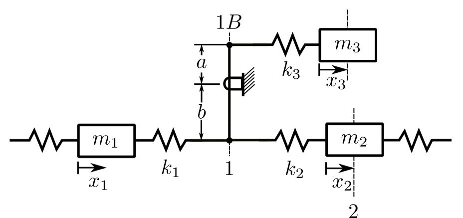
![\[ \{ \mathfrak z\}_1^R = [?] \{ \mathfrak z \}_1^L \]](https://engcourses-uofa.ca/wp-content/ql-cache/quicklatex.com-c86fb71196e71632b78e405d987091d8_l3.png "Rendered by QuickLaTeX.com")
The transfer matrix will include the effect of the branch.
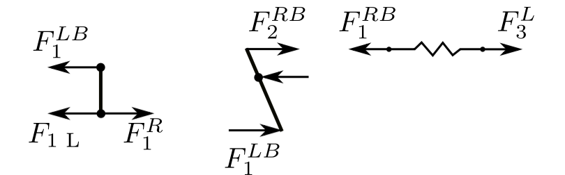
![\[ x_1^B = -\frac{a}{b} x_1 \]](https://engcourses-uofa.ca/wp-content/ql-cache/quicklatex.com-b82270a8f8433dbc1b380cc147312111_l3.png "Rendered by QuickLaTeX.com")
![\[ \sum M_R = F_1^{RB}(a) - F_1^{LB}(b) \]](https://engcourses-uofa.ca/wp-content/ql-cache/quicklatex.com-c7ab69ed90b9a7bd8c5085631f01bf49_l3.png "Rendered by QuickLaTeX.com")
![\[ F_1^{LB} = \frac{a}{b} F_1^{RB} \]](https://engcourses-uofa.ca/wp-content/ql-cache/quicklatex.com-f7cccd8af47db43b7a1402585610c01c_l3.png "Rendered by QuickLaTeX.com")
![\[ \{ \mathfrak z \}_3^L = \begin{bmatrix} 1 & \frac{1}{k_3} \\ 0 & 1 \end{bmatrix} \{ \mathfrak z\}_1^{RB} \]](https://engcourses-uofa.ca/wp-content/ql-cache/quicklatex.com-9f27c1b96b9917360c41813186a9e90e_l3.png "Rendered by QuickLaTeX.com")
![\[ \begin{split} \{ \mathfrak z \}_3^R &= \begin{bmatrix} 1 & 0 \\ -m_3p^2 & 1 \end{bmatrix} \{ \mathfrak z \}_3^L \\&= \begin{bmatrix} 1 & 0 \\ -m_3p^2 & 1 \end{bmatrix} \begin{bmatrix} 1 & \frac{1}{k_3} \\ 0 & 1 \end{bmatrix} \{ \mathfrak z \}_1^{RB} \\&= \begin{bmatrix} 1 & \frac{1}{k_3} \\ -m_3p^2 & 1 - \frac{m_3p^2}{k_3} \end{bmatrix} \{ \mathfrak z \}_1^{RB} \end{split} \]](https://engcourses-uofa.ca/wp-content/ql-cache/quicklatex.com-b5624d940b26d016eba2e8069aa2911b_l3.png "Rendered by QuickLaTeX.com")
Therefore:
![\[ \begin{Bmatrix} x \\ 0 \end{Bmatrix}_3^R = \begin{bmatrix} 1 & \frac{1}{k_3} \\ -m_3p^2 & 1 - \frac{m_3p^2}{k_3} \end{bmatrix} \begin{Bmatrix} x \\ F \end{Bmatrix}_1^{RB} \]](https://engcourses-uofa.ca/wp-content/ql-cache/quicklatex.com-6084de47ab25fc5e9da9dcefc7056bad_l3.png "Rendered by QuickLaTeX.com")
![\[ 0 = -m_3p^2 x_1^{RB} + \Big(1 - \frac{m_3p^2}{k^3} \Big) F_1^{RB} \]](https://engcourses-uofa.ca/wp-content/ql-cache/quicklatex.com-8c0eeea7bcef1b17add1e5784796dc92_l3.png "Rendered by QuickLaTeX.com")
![\[F_1^{RB} = +\frac{m_3p^2x_1^{RB}}{\Big(1 - \frac{m_3p^2}{k_3} \Big)} \]](https://engcourses-uofa.ca/wp-content/ql-cache/quicklatex.com-75c36fbfa9774201c07f2444cc4ae90a_l3.png "Rendered by QuickLaTeX.com")
Therefore:
![\[ F_1^{RB} = -\Big(\frac{a}{b}\Big) \frac{m_3 p^2}{\Big(1 - \frac{m_3p^2}{k^3} \Big)} x_1 \]](https://engcourses-uofa.ca/wp-content/ql-cache/quicklatex.com-7647ecf908cddb5c1529688daeb7a651_l3.png "Rendered by QuickLaTeX.com")
![\[ F_1^{LB} = -\Big(\frac{a}{b}\Big)^2 \frac{m_3 p^2}{\Big(1 - \frac{m_3p^2}{k_3} \Big)} x_1 \]](https://engcourses-uofa.ca/wp-content/ql-cache/quicklatex.com-d32165df4e2d950bd55701693bbabe7b_l3.png "Rendered by QuickLaTeX.com")
![\[ F_1^R = F_1^L + F_1^{LB} \]](https://engcourses-uofa.ca/wp-content/ql-cache/quicklatex.com-b51345565f34d47b561fc72eece8bb6b_l3.png "Rendered by QuickLaTeX.com")
![\[ \{ \mathfrak z \}_1^R = \begin{Bmatrix} x \\ F \end{Bmatrix}_1^R \]](https://engcourses-uofa.ca/wp-content/ql-cache/quicklatex.com-5f0754aeace79bcd2050107ab04212f6_l3.png "Rendered by QuickLaTeX.com")
![\[\begin{Bmatrix} x \\ F \end{Bmatrix}_1^R = \begin{bmatrix} 1 & 0 \\ -\big(\frac{a}{b}\big)^2\frac{m_3p^2}{1-\frac{m_3p^2}{k^3}} & 1 \end{bmatrix}\begin{Bmatrix} x \\ F \end{Bmatrix}_1^L\]](https://engcourses-uofa.ca/wp-content/ql-cache/quicklatex.com-72bc21ce2ea2d08feb08c287a7b2902a_l3.png "Rendered by QuickLaTeX.com")
This now has the “effect” of the branch in it.
![\[\{z\}_2^R = [p]_2[z]_1^2[H]_{1L}^{1R}[z]_0^1[p]_0\{z\}_0^L\]](https://engcourses-uofa.ca/wp-content/ql-cache/quicklatex.com-730b7dbdb1e8b2c837c316106b055d29_l3.png "Rendered by QuickLaTeX.com")
Consider the linear system analog of the torsional one, but with the mass on the other side.
![\[\{\mathfrak z\}_3^{LB} = [p]_3[z]_{1-3}\{\mathfrak z \}_1^{LB}\]](https://engcourses-uofa.ca/wp-content/ql-cache/quicklatex.com-d1993009d11ce8721136d6233551ee31_l3.png "Rendered by QuickLaTeX.com")
![\[\begin{split}\begin{Bmatrix}x \\ 0\end{Bmatrix}_3^{LB} &=\begin{bmatrix} 1 & 0 \\ -m_3p^2 & 1\end{bmatrix}\begin{bmatrix}1 & \frac{1}{k_3} \\ 0 & 1\end{bmatrix}\begin{Bmatrix} x \\ F\end{Bmatrix}_1^{LB} \\&= \begin{bmatrix} 1 & \frac{1}{k_3} \\ -m_3p^2 &1 - \frac{m_3p^2}{k_3}\end{bmatrix}\begin{Bmatrix} x \\ F\end{Bmatrix}_1^{LB}\end{split}\]](https://engcourses-uofa.ca/wp-content/ql-cache/quicklatex.com-9826990ca460646cc7c1ef9c67525e5f_l3.png "Rendered by QuickLaTeX.com")
Therefore:
![\[-m_3p^2x_1^{LB} + \bigg(1-\frac{m_3p^2}{k_3}\bigg)F_1^{LB} = 0\]](https://engcourses-uofa.ca/wp-content/ql-cache/quicklatex.com-7fb18d9b529d54c04ea9f15e6e405b98_l3.png "Rendered by QuickLaTeX.com")
Therefore:
![\[F_1^{LB} = \frac{m_3p^2}{1 - \frac{m_3p^2}{k_3}}x_1^{LB}\]](https://engcourses-uofa.ca/wp-content/ql-cache/quicklatex.com-051cfd2d7546f4d8aefeaa663fa2d651_l3.png "Rendered by QuickLaTeX.com")
Let  :
:
![\[x_1^{LB} = \frac{a}{b}x_1\]](https://engcourses-uofa.ca/wp-content/ql-cache/quicklatex.com-806e2febec9d4b9cf0b05e22db3c2b7c_l3.png "Rendered by QuickLaTeX.com")
Therefore:
![\[\begin{split}x_1^{LB} &= \frac{n_1}{n_1'}x_1^L \\&= \alpha x_1^L\end{split}\]](https://engcourses-uofa.ca/wp-content/ql-cache/quicklatex.com-f8783166120f2c410f5892ccef2572ab_l3.png "Rendered by QuickLaTeX.com")
Therefore:
![\[F_1^{LB} = \frac{m_3p^2\alpha}{1-\frac{m_3p^2}{k_3}}x_1^L\]](https://engcourses-uofa.ca/wp-content/ql-cache/quicklatex.com-7a79195b32c6ad802f2c37a88b372d0c_l3.png "Rendered by QuickLaTeX.com")
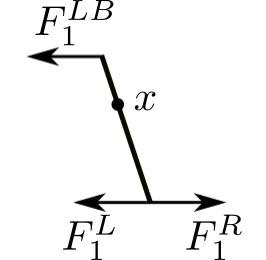
![\[\begin{split}+\circlearrowleft \sum M_x &= 0 \\&= F_1^{LB}a + F_1^Rb - F_1^Lb\end{split}\]](https://engcourses-uofa.ca/wp-content/ql-cache/quicklatex.com-e4ed0532a6778ea27d77b10f78882160_l3.png "Rendered by QuickLaTeX.com")
Therefore:
![\[F_1^R = -F_1^{LB}\alpha +F_1^L\]](https://engcourses-uofa.ca/wp-content/ql-cache/quicklatex.com-2f7a7f8b010fa500d01999198b6aa6d1_l3.png "Rendered by QuickLaTeX.com")
![\[x_1^R = x_1^L\]](https://engcourses-uofa.ca/wp-content/ql-cache/quicklatex.com-0ea2fa1b46030f34a056bbde3aeba7d5_l3.png "Rendered by QuickLaTeX.com")
Therefore:
![\[\begin{Bmatrix} x \\ F \end{Bmatrix}_1^R = \begin{bmatrix} 1 & 0 \\ -\frac{m_3p^2}{1-\frac{m_3p^2\alpha^2}{k^3}} & 1 \end{bmatrix}\begin{Bmatrix} x \\ F \end{Bmatrix}_1^L\]](https://engcourses-uofa.ca/wp-content/ql-cache/quicklatex.com-44efb48429ded3969347fc1d110340cb_l3.png "Rendered by QuickLaTeX.com")
By analogy, the torsional system is:
![\[\begin{Bmatrix} \theta \\ T \end{Bmatrix}_1^R = \begin{bmatrix} 1 & 0 \\ -\frac{J_3p^2\alpha^2}{1-\frac{J_3p^2}{k_3}} & 1 \end{bmatrix}\begin{Bmatrix} \theta \\ T \end{Bmatrix}_1^L\]](https://engcourses-uofa.ca/wp-content/ql-cache/quicklatex.com-afc6cdd8b2ba9a6ff39545f9b1bdadfc_l3.png "Rendered by QuickLaTeX.com")
The transfer matrix approach can be extended to handle geared and branched systems. We can derive the results from scratch or use the analog of the translational systems.
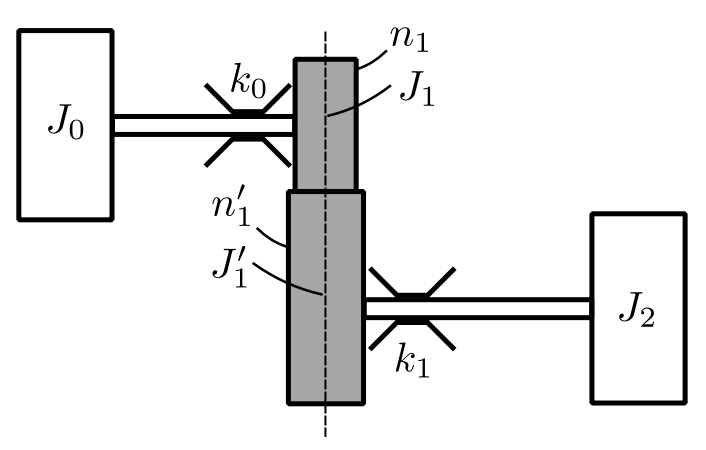
We wish to find  in terms of
  :
:
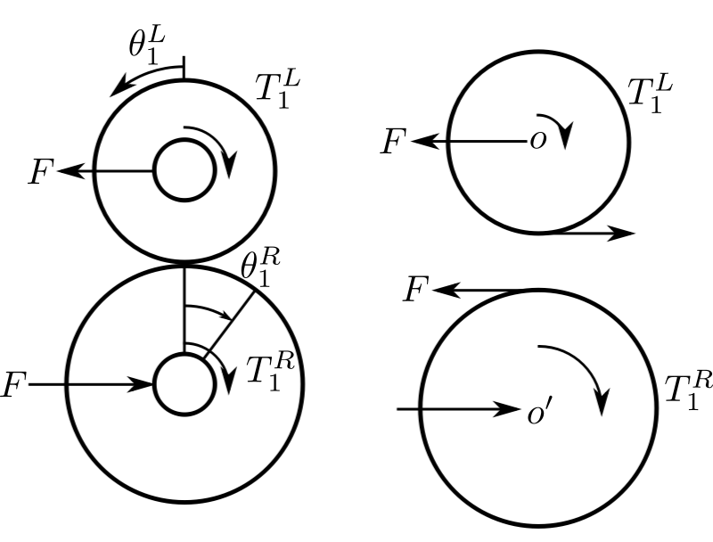
![\[T_1^L = F_{n_1}\]](https://engcourses-uofa.ca/wp-content/ql-cache/quicklatex.com-8fc7a1897d38c7e3f129bbbf42498da7_l3.png "Rendered by QuickLaTeX.com")
![\[T_1^R = F_{n_1'}\]](https://engcourses-uofa.ca/wp-content/ql-cache/quicklatex.com-e751a3ff89c13f32ec40ad3cacb7be00_l3.png "Rendered by QuickLaTeX.com")
![\[\theta_1^Ln_1 = \theta_1^Rn_1'\]](https://engcourses-uofa.ca/wp-content/ql-cache/quicklatex.com-cd34fe7e6aec15b3ccc9cb2c7385b2b3_l3.png "Rendered by QuickLaTeX.com")
Therefore:
![\[T_1^R = T_1^L\frac{n_1'}{N_1}\]](https://engcourses-uofa.ca/wp-content/ql-cache/quicklatex.com-173d36ea1f84f360b72a60e055370c43_l3.png "Rendered by QuickLaTeX.com")
![\[\theta_1^R = \frac{n_1}{n_1'}\theta_1^L \]](https://engcourses-uofa.ca/wp-content/ql-cache/quicklatex.com-35308b63fa6e123e5ca2539bed466e3f_l3.png "Rendered by QuickLaTeX.com")
set  :
:
![\[\theta_1^R= \alpha\theta_1^L\]](https://engcourses-uofa.ca/wp-content/ql-cache/quicklatex.com-90be94f4c44072a02fad46c4ccdd15f8_l3.png "Rendered by QuickLaTeX.com")
![\[\{\mathfrak z\}_1^R = \begin{bmatrix} \alpha & 0 \\ 0 & \frac{1}{\alpha}\end{bmatrix}\{\mathfrak z\}_1^L\]](https://engcourses-uofa.ca/wp-content/ql-cache/quicklatex.com-a95b5f96e70ee9968e328974dd3712c4_l3.png "Rendered by QuickLaTeX.com")
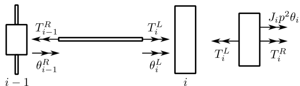
We can also include the effect of the inertia of the gears:
![\[\begin{split}+\circlearrowleft \sum M_0 &= J_1\ddot\theta_1^L \\&= -T_1^L + F_{n_1}\end{split}\]](https://engcourses-uofa.ca/wp-content/ql-cache/quicklatex.com-241bc93a7e5c51e5a3753b1ceb028eb3_l3.png "Rendered by QuickLaTeX.com")
![\[\begin{split}+\circlearrowright \sum M_0' &= J'_1\ddot\theta_1^R \\&= T_1^R - F_{n_1'}\end{split}\]](https://engcourses-uofa.ca/wp-content/ql-cache/quicklatex.com-18c111e38033849e9a55a44372d69142_l3.png "Rendered by QuickLaTeX.com")
![\[F = -\frac{J_1'\ddot\theta_1^R}{n_1} + T_1^R\]](https://engcourses-uofa.ca/wp-content/ql-cache/quicklatex.com-7eeb208c25f4c3bdf0c09fde00b7cc64_l3.png "Rendered by QuickLaTeX.com")
Therefore:
![\[J_1\ddot\theta_1^L = -T_1^L - J_1'\ddot\theta_1^R\frac{n_1}{n_1'}+T_1^R\frac{n_1}{n_1'}\]](https://engcourses-uofa.ca/wp-content/ql-cache/quicklatex.com-4d7d035831cc98c34e3a76254078b7f0_l3.png "Rendered by QuickLaTeX.com")
![\[J_1\ddot\theta_1^L + J_1'\ddot\theta_1^R\frac{n_1}{n_1'} = - T_1^L + T_1^R\frac{n_1}{n_1'}\]](https://engcourses-uofa.ca/wp-content/ql-cache/quicklatex.com-715160fcae64c910cbb6a5a44a10ec93_l3.png "Rendered by QuickLaTeX.com")
Again we assume  . Therefore:
![\[-p^2\bigg(J_1\theta_1^L + J_1'\frac{n_1}{n_1'}\theta_1^R\bigg) = -T_1^L + T_1^R\frac{n_1}{n_1'}\]](https://engcourses-uofa.ca/wp-content/ql-cache/quicklatex.com-c1b5ddcfa45ac366f1f1c3a633fa23d5_l3.png "Rendered by QuickLaTeX.com")
![\[-p^2(J_1\theta_1^L + J_1'\alpha^2)\theta_1^L = -T_1^L + \alpha T_1^R \]](https://engcourses-uofa.ca/wp-content/ql-cache/quicklatex.com-f10ba7d24088e942c4922aa22927710d_l3.png "Rendered by QuickLaTeX.com")
Therefore:
![\[T_1^R = \frac{1}{\alpha}T_1^L - p^2\bigg(\frac{J_1}{\alpha} + J_1'\alpha\bigg)\theta_1^L\]](https://engcourses-uofa.ca/wp-content/ql-cache/quicklatex.com-66f333c00c018227090d5767941086b0_l3.png "Rendered by QuickLaTeX.com")
Therefore:
![\[\{\mathfrak z\}_1^R = \begin{bmatrix} \alpha & 0 \\ -p^2\bigg(\frac{J_1}{\alpha} + J_1'\alpha\bigg) & \frac{1}{\alpha}\end{bmatrix}\{\mathfrak z\}_1^L\]](https://engcourses-uofa.ca/wp-content/ql-cache/quicklatex.com-2cdb7cca63264b0c6c0f2c5b517f0a14_l3.png "Rendered by QuickLaTeX.com")
![\[\{\mathfrak z\}_1^L = [z]_{0-1}[p]_0\{\mathfrak z\}_0^L\]](https://engcourses-uofa.ca/wp-content/ql-cache/quicklatex.com-2e0c7b148576f3aca503612f6a0f46ed_l3.png "Rendered by QuickLaTeX.com")
![\[\{\mathfrak z\}_2^R = [p]_2[z]_{1 \to 2}\{\mathfrak z\}_1^R\]](https://engcourses-uofa.ca/wp-content/ql-cache/quicklatex.com-57bb6ad49c9692502303f3a35613a4f3_l3.png "Rendered by QuickLaTeX.com")
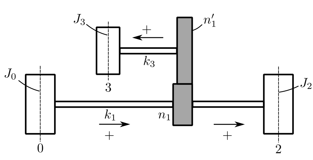
To determine the relationship between and  , consider the branch (B).
![\[\{\mathfrak z\}_3^L = [p]_3[z]_{1-3}\{\mathfrak z\}_1^{LB}\]](https://engcourses-uofa.ca/wp-content/ql-cache/quicklatex.com-1acc965888e0c9a2ed8c22b0740bc9aa_l3.png "Rendered by QuickLaTeX.com")
![\[\begin{split}\begin{Bmatrix}\theta \\ 0 \end{Bmatrix}_3^L &= \begin{bmatrix} 1 & 0 \\ -J_3p^2 & 1 \end{bmatrix}\begin{bmatrix} 1 & \frac{1}{k_3} \\ 0 & 1 \end{bmatrix}\{\mathfrak z\}_1^{LB} \\&= \begin{bmatrix} 1 & \frac{1}{k_3} \\ -J_3p^2 & 1 - \frac{J_3p^2}{k_3}\end{bmatrix}\{\mathfrak z\}_1^{LB}\end{split}\]](https://engcourses-uofa.ca/wp-content/ql-cache/quicklatex.com-12df0c0c2a0627fb31becc069bed25be_l3.png "Rendered by QuickLaTeX.com")
Therefore:
![\[-J_3p^2\theta_1^B+ \bigg(1-\frac{J_3p^2}{k_3}\bigg)T_1^{LB} = 0\]](https://engcourses-uofa.ca/wp-content/ql-cache/quicklatex.com-d8633baeb5d23adf678419f68e79b9cc_l3.png "Rendered by QuickLaTeX.com")
![\[T_1^{LB}=\frac{J_3p^2}{1-\frac{J_3p^2}{k_3}}\theta_1^B\]](https://engcourses-uofa.ca/wp-content/ql-cache/quicklatex.com-939350ad6ee370dd0a2639ea471fb5c2_l3.png "Rendered by QuickLaTeX.com")
If we take counterclockwise as positive with increasing numbers as shown above then viewing the gears from the left gives.
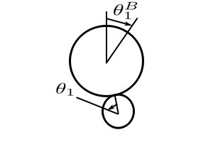
![\[\theta_1^B = \alpha\theta_1\]](https://engcourses-uofa.ca/wp-content/ql-cache/quicklatex.com-af2532dd924b23070895e6f04d2d4511_l3.png "Rendered by QuickLaTeX.com")
Therefore:
![\[T_1^{LB} = \frac{J_3p^2\alpha}{1-\frac{J_3p^2}{k_3}}\theta_1\]](https://engcourses-uofa.ca/wp-content/ql-cache/quicklatex.com-b85dd6f34eb332a8857776b0efe25c06_l3.png "Rendered by QuickLaTeX.com")
Consider a free body diagram of the gears viewed from the left:
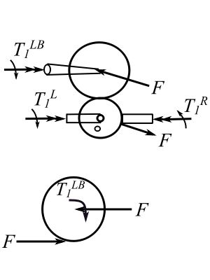
![\[+\circlearrowleft\sum M_0 = -T_1^L+T_1^R-T_1^{LB}+F(n_1+n'_1)\]](https://engcourses-uofa.ca/wp-content/ql-cache/quicklatex.com-2d10c7b929366091e5f737b64f55a850_l3.png "Rendered by QuickLaTeX.com")
Therefore:
![\[T_1^R=T_1^L+T_1{LB}-F(n_1+n'_1)\]](https://engcourses-uofa.ca/wp-content/ql-cache/quicklatex.com-be8b47d387c60e9cb9a164a0146ef885_l3.png "Rendered by QuickLaTeX.com")
![\[T_1^R = T_1^L-T_1^{LB}\alpha\]](https://engcourses-uofa.ca/wp-content/ql-cache/quicklatex.com-7bc9f8cbd7ebeb90be0b4e55aca49e21_l3.png "Rendered by QuickLaTeX.com")
Therefore:
![\[T_1^{LB}=Fn'_1\]](https://engcourses-uofa.ca/wp-content/ql-cache/quicklatex.com-c58b390e17b8f59992636871e13598ee_l3.png "Rendered by QuickLaTeX.com")
Therefore:
![\[T_1^R=T_1^L-\frac{J_3p^2\alpha^2}{1-\frac{J_3p^2}{k_3}}\theta_1\]](https://engcourses-uofa.ca/wp-content/ql-cache/quicklatex.com-fef639a89ff0fe5b8a80c8d04853165e_l3.png "Rendered by QuickLaTeX.com")
![\[\begin{split}\begin{Bmatrix}\theta \\T \end{Bmatrix}_1^R &= \begin{bmatrix} 1 & 0 \\ -\frac{J_3p^2\alpha^2}{1-\frac{J_3p^2}{k_3}} & 1\end{bmatrix}\begin{Bmatrix} \theta \\ T\end{Bmatrix}_1^L \\&= [H]\{\mathfrak z\}_1^L\end{split}\]](https://engcourses-uofa.ca/wp-content/ql-cache/quicklatex.com-f77b1face6bceebf940485636ae5600b_l3.png "Rendered by QuickLaTeX.com")
Therefore the effect of the branch is embodied in the  term.
term.
Example 3
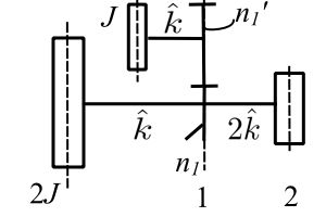
![\[\frac{n_1}{n'_1} = \frac{1}{2}\]](https://engcourses-uofa.ca/wp-content/ql-cache/quicklatex.com-309fece4f69dc29730ed77dfd7d7c4ba_l3.png "Rendered by QuickLaTeX.com")
Again write down the state vectors and transfers matricies also nondimensionalize by dividing the torques by  .
.
![\[\begin{split}\{\mathfrak z\}_3^L &= [Z]_{1-3}\{\mathfrak z\}_1^{LB} \\&= \begin{bmatrix} 1 & 1 \\ 0 & 1\end{bmatrix}\begin{Bmatrix} \theta \\ \bar T \end{Bmatrix}_1^{LB}\end{split}\]](https://engcourses-uofa.ca/wp-content/ql-cache/quicklatex.com-97627c37524453639107a20c2e1720e6_l3.png "Rendered by QuickLaTeX.com")
We need this only to calculate the mode shape.
![\[\{\mathfrak z\}_2^R = [p]_2[Z]_{1-2}[H]_{1L}^{1R}[Z]_{0-1}[p]_0\{\mathfrak z\}_0^L\]](https://engcourses-uofa.ca/wp-content/ql-cache/quicklatex.com-fe539d40473f12ca37eb370fc18e0553_l3.png "Rendered by QuickLaTeX.com")
![\[\begin{split}[p]_0 &= \begin{bmatrix} 1 & 0 \\ -\frac{2p^2J}{k} & 1\end{bmatrix}[Z]_{0-1} \\&= \begin{bmatrix} 1 & 1 \\ 0 & 1\end{bmatrix}\end{split}\]](https://engcourses-uofa.ca/wp-content/ql-cache/quicklatex.com-7ecccf0b09723c5ddd8acb94b2514ba4_l3.png "Rendered by QuickLaTeX.com")
![\[\begin{split}[H]_{1L}^{1R} &= \begin{bmatrix}1 & 0 \\ -\frac{p^2J}{4k(1-\frac{p^2J}{k})} & 1 \end{bmatrix}[Z]_{1-2} \\&= \begin{bmatrix}1 & 0.5 \\ 0 & 1 \end{bmatrix}\end{split}\]](https://engcourses-uofa.ca/wp-content/ql-cache/quicklatex.com-c299f5dd0878de8b38a8f273e419e687_l3.png "Rendered by QuickLaTeX.com")
![\[[p]_2 = \begin{bmatrix}1 & 0 \\ -\frac{p^2J}{k} & 1 \end{bmatrix}\]](https://engcourses-uofa.ca/wp-content/ql-cache/quicklatex.com-408c992e1b77beea13bca9d3407464c2_l3.png "Rendered by QuickLaTeX.com")
![\[\begin{split}x_3^B &= x_1^{LB} + \frac{1}{k_3}F_1^{LB} \\&= \alpha x_1 + \frac{1}{k_3}F_1^{LB} \\&= \alpha x_1 + \frac{\frac{m_3}{k_3}p^2\alpha}{1-\frac{m_3p^2}{k_3}}x_1 \\&= \alpha x_1\bigg[1+\frac{\frac{m_3}{k_3}p^2}{1-\frac{m_3p^2}{k_3}}\bigg] \\&=\alpha x_1\frac{1}{1-\frac{m_3p^2}{k_3}} \\&= \frac{\alpha x_1}{1-\frac{m_3p^2}{k_3}}\end{split}\]](https://engcourses-uofa.ca/wp-content/ql-cache/quicklatex.com-55eb3184707935fb517515539f313066_l3.png "Rendered by QuickLaTeX.com")
For this case  :
:
![\[\theta_3^B = \frac{\frac{1}{2}}{1 - \frac{p^2J}{k}}\theta_1\]](https://engcourses-uofa.ca/wp-content/ql-cache/quicklatex.com-a79d97a067243f6328208454a7ca54db_l3.png "Rendered by QuickLaTeX.com")
Now begin by selecting  :
:
![\[\{\mathfrak z\}_0^R = \begin{bmatrix} 1 & 0 \\ -1 &1\end{bmatrix}\begin{bmatrix} \theta \\ 0\end{bmatrix}_0^L\]](https://engcourses-uofa.ca/wp-content/ql-cache/quicklatex.com-95e4833fec8eb2e58e0ebea25a90d2d3_l3.png "Rendered by QuickLaTeX.com")
![\[\begin{split}\{\mathfrak z\}_1^L &= \begin{bmatrix} 0 & 1 \\ -1 &1\end{bmatrix}\begin{bmatrix} \theta \\ 0\end{bmatrix}_0^L \\&=\begin{bmatrix} 1 & 1\\0&1\end{bmatrix}\begin{bmatrix}1 & 0 \\ -1& 1\end{bmatrix}\begin{bmatrix}\theta \\ 0 \end{bmatrix}_0^L\end{split}\]](https://engcourses-uofa.ca/wp-content/ql-cache/quicklatex.com-48e8df34a69341235ea0d2366f0f692f_l3.png "Rendered by QuickLaTeX.com")
![\[\begin{split}\{\mathfrak z\}_1^R &= \begin{bmatrix} 0 & 1 \\ -1 &0.75\end{bmatrix}\begin{bmatrix} \theta \\0\end{bmatrix}_0^L \\&=\begin{bmatrix} 1 &0\\-0.25&1\end{bmatrix}\begin{bmatrix}0 & 1 \\ -1& 1\end{bmatrix}\begin{bmatrix}\theta \\ 0 \end{bmatrix}_0^L\end{split}\]](https://engcourses-uofa.ca/wp-content/ql-cache/quicklatex.com-6db2585bbbd187b67df4368db85e0627_l3.png "Rendered by QuickLaTeX.com")
![\[\begin{split}\{\mathfrak z\}_2^L &= \begin{bmatrix} -0.5 & 1.375 \\ -1 &0.75\end{bmatrix}\begin{bmatrix} \theta \\0\end{bmatrix}_0^L \\&=\begin{bmatrix} 1 & 0.5\\0&1\end{bmatrix}\begin{bmatrix}0 & 1 \\ -1& 0.75\end{bmatrix}\begin{bmatrix}\theta \\ 0 \end{bmatrix}_0^L\end{split}\]](https://engcourses-uofa.ca/wp-content/ql-cache/quicklatex.com-4f48c0e79ff4ac08682b056016b90d14_l3.png "Rendered by QuickLaTeX.com")
![\[\begin{split}\{\mathfrak z\}_2^R &= \begin{bmatrix} -0.5 & 1.375 \\ -0.75 & 0.0625\end{bmatrix}\begin{bmatrix} \theta \\ 0 \end{bmatrix} \\&=\begin{bmatrix} 1 & 0 \\ -0.5&1\end{bmatrix}\begin{bmatrix}-0.5 & 1.375 \\ -1 & 0.75 \end{bmatrix}\begin{bmatrix} \theta \\ 0\end{bmatrix}_0^L\end{split}\]](https://engcourses-uofa.ca/wp-content/ql-cache/quicklatex.com-c8e71f2fa44120259bb1a84b59034f89_l3.png "Rendered by QuickLaTeX.com")
Therefore:
![\[\begin{Bmatrix} \theta_0 \\ \theta_2 \\ \theta_3\end{Bmatrix} = \begin{Bmatrix} 1 \\ -0.5 \\ 0 \end{Bmatrix}\]](https://engcourses-uofa.ca/wp-content/ql-cache/quicklatex.com-ee153cd6d39ce25757c7572adcb06d0f_l3.png "Rendered by QuickLaTeX.com")
Now try  :
:
![\[\{\mathfrak z\}_0^R = \begin{bmatrix} 1 & 0 \\ -1.6 &1\end{bmatrix}\begin{bmatrix} \theta \\ 0\end{bmatrix}_0^L\]](https://engcourses-uofa.ca/wp-content/ql-cache/quicklatex.com-719aff240786d7211e96dac843c502ea_l3.png "Rendered by QuickLaTeX.com")
![\[\begin{split}\{\mathfrak z\}_1^L &= \begin{bmatrix} -0.6 & 1 \\ -1.6 &1\end{bmatrix}\begin{bmatrix} \theta \\0\end{bmatrix}_1^L \\&=\begin{bmatrix} 1 & 1\\0&1\end{bmatrix}\begin{bmatrix}1 & 0 \\ -1.6& 1\end{bmatrix}\begin{bmatrix}\theta \\ 0 \end{bmatrix}_1^L\end{split}\]](https://engcourses-uofa.ca/wp-content/ql-cache/quicklatex.com-512d0e682d4c2dcf4ec95016210ff76c_l3.png "Rendered by QuickLaTeX.com")
![\[\begin{split}\{\mathfrak z\}_1^R &= \begin{bmatrix} -0.6 & 1 \\ -1 &0\end{bmatrix}\begin{bmatrix} \theta \\0\end{bmatrix}_1^L \\&=\begin{bmatrix} 1 & 0\\-1&1\end{bmatrix}\begin{bmatrix}-0.6 & 1 \\ -1.6& 1\end{bmatrix}\begin{bmatrix}\theta \\ 0 \end{bmatrix}_1^L\end{split}\]](https://engcourses-uofa.ca/wp-content/ql-cache/quicklatex.com-1f63b58f1eb3cd08f8c7f620acc9b0a9_l3.png "Rendered by QuickLaTeX.com")
![\[\begin{split}\{\mathfrak z\}_2^L &= \begin{bmatrix} -1.1 & 1 \\ -1 &0\end{bmatrix}\begin{bmatrix} \theta \\0\end{bmatrix}_1^L \\&=\begin{bmatrix} 1 & 0.5\\0&1\end{bmatrix}\begin{bmatrix}-0.6 & 1 \\ -1& 0\end{bmatrix}\begin{bmatrix}\theta \\ 0 \end{bmatrix}_1^L\end{split}\]](https://engcourses-uofa.ca/wp-content/ql-cache/quicklatex.com-4040406618e6641ae3c5a5f7bf8e3b56_l3.png "Rendered by QuickLaTeX.com")
![\[\begin{split}\{\mathfrak z\}_2^R &= \begin{bmatrix} -1.1& 1 \\ -0.12 & -0.5\end{bmatrix}\begin{bmatrix} \theta \\ 0 \end{bmatrix} \\&=\begin{bmatrix} 1 & 0 \\ -0.8&1\end{bmatrix}\begin{bmatrix}-1.1 & 1\\ -1 & 0 \end{bmatrix}\begin{bmatrix} \theta \\ 0\end{bmatrix}\end{split}\]](https://engcourses-uofa.ca/wp-content/ql-cache/quicklatex.com-cf3b46d0bf51d5386ef1aebe88a32014_l3.png "Rendered by QuickLaTeX.com")
![\[\theta_3 = \frac{\frac{1}{2}}{1-0.8}(1) = -2.5\]](https://engcourses-uofa.ca/wp-content/ql-cache/quicklatex.com-0776703fe2259a42e47af1efd9517c9b_l3.png "Rendered by QuickLaTeX.com")
![\[\begin{Bmatrix} \theta_0 \\ \theta_2 \\ \theta_3\end{Bmatrix} = \begin{Bmatrix} 1 \\ -1.1 \\ -2.5 \end{Bmatrix}\]](https://engcourses-uofa.ca/wp-content/ql-cache/quicklatex.com-aac26cd52d905024cf0bae56f4be1f5e_l3.png "Rendered by QuickLaTeX.com")
Now try  :
:
![\[\{\mathfrak z\}_1^R = \begin{bmatrix} 1 & 0 \\ -1.7 &1\end{bmatrix}\begin{bmatrix} \theta \\ 0\end{bmatrix}_0^L\]](https://engcourses-uofa.ca/wp-content/ql-cache/quicklatex.com-becdbaf2cf39f1f130e6245f8e03ea00_l3.png "Rendered by QuickLaTeX.com")
![\[\begin{split}\{\mathfrak z\}_1^L &= \begin{bmatrix} -0.7 & 1 \\ -1.7 &1\end{bmatrix}\begin{bmatrix} \theta \\0\end{bmatrix} \\&=\begin{bmatrix} 1 & 1\\0&1\end{bmatrix}\begin{bmatrix}1 & 0 \\ -1.7& 1\end{bmatrix}\begin{bmatrix}\theta \\ 0 \end{bmatrix}\end{split}\]](https://engcourses-uofa.ca/wp-content/ql-cache/quicklatex.com-7dcfeabbdd46ff721498c2bbcfd11c0a_l3.png "Rendered by QuickLaTeX.com")
![\[\begin{split}\{\mathfrak z\}_1^R &= \begin{bmatrix} -0.7& 1 \\ -0.7083 &-0.1467\end{bmatrix}\begin{bmatrix} \theta \\0\end{bmatrix}\\&=\begin{bmatrix} 1 & 0\\-1.1467&1\end{bmatrix}\begin{bmatrix}-0.7 & 1 \\ -1.7& 1\end{bmatrix}\begin{bmatrix}\theta \\ 0 \end{bmatrix}\end{split}\]](https://engcourses-uofa.ca/wp-content/ql-cache/quicklatex.com-a135ee533b40700b7f4b7c5740b8a886_l3.png "Rendered by QuickLaTeX.com")
![\[\begin{split}\{\mathfrak z\}_2^L &= \begin{bmatrix} -1.0542& 0.9267 \\ -0.7083 & -0.1467\end{bmatrix}\begin{bmatrix} \theta \\0\end{bmatrix}_0^L \\&=\begin{bmatrix} 1 & 0.5\\0&1\end{bmatrix}\begin{bmatrix}-0.7 & 1 \\ -0.7083& -0.1467\end{bmatrix}\begin{bmatrix}\theta \\ 0 \end{bmatrix}_0^L\end{split}\]](https://engcourses-uofa.ca/wp-content/ql-cache/quicklatex.com-7e2801ab75db5e745cfc4731f1a6aac3_l3.png "Rendered by QuickLaTeX.com")
![\[\begin{split}\{\mathfrak z\}_2^R &= \begin{bmatrix} -1.0542& 0.9267\\ 0.1877 \end{bmatrix}\begin{bmatrix} \theta \\ 0 \end{bmatrix}_0^L \\&=\begin{bmatrix} 1 & 0 \\ -0.85&1\end{bmatrix}\begin{bmatrix}-1.0542 & 0.9267\\ -0.7083 & -0.1467 \end{bmatrix}\begin{bmatrix} \theta \\ 0\end{bmatrix}_0^L\end{split}\]](https://engcourses-uofa.ca/wp-content/ql-cache/quicklatex.com-2f40c6580da3e4bac9bc345737fe9e01_l3.png "Rendered by QuickLaTeX.com")
![\[\theta_3 = \frac{\frac{1}{2}}{1-0.85}\theta_1 = \frac{\frac{1}{2}(-0.7)}{0.15}\]](https://engcourses-uofa.ca/wp-content/ql-cache/quicklatex.com-389e1c7430cf9f42beb749d9c2b3af18_l3.png "Rendered by QuickLaTeX.com")
![\[\begin{Bmatrix} \theta_0 \\ \theta_2 \\ \theta_3\end{Bmatrix} = \begin{Bmatrix} 1 \\ -1.0542 \\ -2.33 \end{Bmatrix}\]](https://engcourses-uofa.ca/wp-content/ql-cache/quicklatex.com-e37a8c0a823940d52018cd6c03004fff_l3.png "Rendered by QuickLaTeX.com")
Now try  :
:
![\[\{\mathfrak z\}_1^R = \begin{bmatrix} 1 & 0 \\ -4 &1\end{bmatrix}\begin{bmatrix} \theta \\ 0\end{bmatrix}_1^L\]](https://engcourses-uofa.ca/wp-content/ql-cache/quicklatex.com-1ae23b3c245c9d69f0d118ad6987ec37_l3.png "Rendered by QuickLaTeX.com")
![\[\begin{split}\{\mathfrak z\}_1^L &= \begin{bmatrix} -3 & 1 \\ -4 &1\end{bmatrix}\begin{bmatrix} \theta \\0\end{bmatrix}_1^L \\&=\begin{bmatrix} 1 & 1\\0&1\end{bmatrix}\begin{bmatrix}1 & 0 \\ -4& 1\end{bmatrix}\begin{bmatrix}\theta \\ 0 \end{bmatrix}_1^L\end{split}\]](https://engcourses-uofa.ca/wp-content/ql-cache/quicklatex.com-95c757a2d9f2fcc12045f1b7b3ba2f59_l3.png "Rendered by QuickLaTeX.com")
![\[\begin{split}\{\mathfrak z\}_1^R &= \begin{bmatrix} -3& 1 \\ -\frac{11}{2}&\frac{3}{2}\end{bmatrix}\begin{bmatrix} \theta \\0\end{bmatrix}_1^L \\&=\begin{bmatrix} 1 & 0\\\frac{1}{2}&1\end{bmatrix}\begin{bmatrix}-3 & 1 \\ -4& 1\end{bmatrix}\begin{bmatrix}\theta \\ 0 \end{bmatrix}_1^L\end{split}\]](https://engcourses-uofa.ca/wp-content/ql-cache/quicklatex.com-311ddf7300d1707f478e51feb29c6c6b_l3.png "Rendered by QuickLaTeX.com")
![\[\begin{split}\{\mathfrak z\}_2^L &= \begin{bmatrix} -\frac{23}{4}& \frac{7}{4} \\ -\frac{11}{2} &\frac{3}{2}\end{bmatrix}\begin{bmatrix} \theta \\0\end{bmatrix}_1^L \\&=\begin{bmatrix} 1 & \frac{1}{2}\\0&1\end{bmatrix}\begin{bmatrix}-3 & 1 \\ -\frac{11}{2}& \frac{3}{2}\end{bmatrix}\begin{bmatrix}\theta \\ 0 \end{bmatrix}_1^L\end{split}\]](https://engcourses-uofa.ca/wp-content/ql-cache/quicklatex.com-ae359d17a7bc8f73aeae89586eb1573f_l3.png "Rendered by QuickLaTeX.com")
![\[\begin{split}\{\mathfrak z\}_2^R &= \begin{bmatrix} -\frac{23}{4}& \frac{7}{4}\\ 6 &-2 \end{bmatrix}\begin{bmatrix} \theta \\ 0 \end{bmatrix} \\&=\begin{bmatrix} 1 & 0 \\ -2&1\end{bmatrix}\begin{bmatrix}-\frac{23}{4}& \frac{7}{4}\\ -\frac{11}{2} & \frac{3}{2} \end{bmatrix}\begin{bmatrix} \theta \\ 0\end{bmatrix}_1^L\end{split}\]](https://engcourses-uofa.ca/wp-content/ql-cache/quicklatex.com-69100cdee46050b3fbd4325e9e9e0c99_l3.png "Rendered by QuickLaTeX.com")
![\[\begin{Bmatrix} \theta_0 \\ \theta_2 \\ \theta_3\end{Bmatrix} = \begin{Bmatrix} 1 \\ -\frac{23}{4} \\ -\frac{3}{2} \end{Bmatrix}\]](https://engcourses-uofa.ca/wp-content/ql-cache/quicklatex.com-3edef037805577f1ec8db2ce5f138a9c_l3.png "Rendered by QuickLaTeX.com")
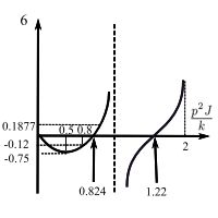
The coefficient  as
as  . This is because of the transfer function where the branch occurs. This hold for any number of branches. If the main shaft is excited at the natural frequency of any one of the branches, the amplitude at the branch point is zero and the branch acts as a vibration absorber.
We can extend the transfer matrices to beams and to include a more realistic effect for shafts etc.
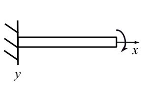
Shafts
![\[ \begin{split} T &= \mu I\frac{\partial\theta}{\partial x} \\ &= \frac{\hat{k}L}{I}I\frac{\partial\theta}{\partial x} \end{split} \]](https://engcourses-uofa.ca/wp-content/ql-cache/quicklatex.com-ce0fd6a120dde47ef6a0edbdf54392ba_l3.png "Rendered by QuickLaTeX.com")
![\[ \begin{Bmatrix} z \end{Bmatrix}_1 = \begin{Bmatrix} \theta \\ T \end{Bmatrix}_1 \]](https://engcourses-uofa.ca/wp-content/ql-cache/quicklatex.com-e48ad9dfc897e1b8b587a86823dd508d_l3.png "Rendered by QuickLaTeX.com")
![\[ \gamma = p\sqrt{\frac{J}{\hat{k}}} \quad \leftarrow \text{ total moment of inertia of rod} \]](https://engcourses-uofa.ca/wp-content/ql-cache/quicklatex.com-38760a19b583f733126cd7dc99ec6ca3_l3.png "Rendered by QuickLaTeX.com")
![\[ \theta = A\cos{\gamma x}{L} + B\sin{\gamma x}{L} \]](https://engcourses-uofa.ca/wp-content/ql-cache/quicklatex.com-5ad33d5013d9806e7a4d95fad22e9775_l3.png "Rendered by QuickLaTeX.com")
at  therefore
at 
![\[ T = \hat{k} L \Big[ -\frac{\gamma\theta_1}{L}\sin{\frac{\gamma x}{L}} + \frac{B\gamma}{L}\cos{\frac{\gamma x}{L}} \Big] \]](https://engcourses-uofa.ca/wp-content/ql-cache/quicklatex.com-387ddad094758567ec9cb58f3530a2c6_l3.png "Rendered by QuickLaTeX.com")
Therefore:
![\[ \begin{split} T_1 &= B\hat{k}\gamma \\ B &= \frac{T_1}{\hat{k}\gamma} \end{split} \]](https://engcourses-uofa.ca/wp-content/ql-cache/quicklatex.com-2c5307660d30d2c226a4f8c36f52a956_l3.png "Rendered by QuickLaTeX.com")
Therefore:
![\[ \theta = \theta_1 \cos{\frac{\gamma x}{L}} + \frac{T_1}{k \gamma}\sin{\frac{\gamma x}{L}} \]](https://engcourses-uofa.ca/wp-content/ql-cache/quicklatex.com-5df1dc951922feddcd016b19e314940f_l3.png "Rendered by QuickLaTeX.com")
![\[ \begin{split} T &= -\gamma \hat{k} \theta_1 \sin{\frac{\gamma x}{L}} + \frac{T_1}{\hat{k}\gamma} \frac{\gamma}{L} \hat{k}L\cos{\frac{\gamma x}{L}} \\ T&= -\gamma \hat{k} \theta_1 \sin{\frac{\gamma x}{L}} + T_1\cos{\frac{\gamma x}{L}} \end{split} \]](https://engcourses-uofa.ca/wp-content/ql-cache/quicklatex.com-65f15a062a793e10d5806acb30ff7b2c_l3.png "Rendered by QuickLaTeX.com")
evaluate these at 
![\[ \begin{split} \theta_2 &= \theta_1 \cos{\gamma} + \frac{T_1}{\hat{k}\gamma} \sin{\gamma} \\ T_2 &= -\gamma \hat{k} \theta_1 \sin{\gamma} + T_1 \cos{\gamma} \end{split} \]](https://engcourses-uofa.ca/wp-content/ql-cache/quicklatex.com-7c3309ba8b2f6750a03932ae26561065_l3.png "Rendered by QuickLaTeX.com")
Therefore:
![\[ \begin{pmatrix} \theta \\ T \end{pmatrix}_2 = \begin{bmatrix} \cos{\gamma} && \frac{\sin{\gamma}}{\hat{k}\gamma} \\ -\gamma \hat{k} \sin{\gamma} && \cos{\gamma} \end{bmatrix} \]](https://engcourses-uofa.ca/wp-content/ql-cache/quicklatex.com-6f81e5c91e6bbe2435e5301dd38c8940_l3.png "Rendered by QuickLaTeX.com")
If the moment of inertia of the shaft is small  and the field matrix becomes
![\[ \begin{bmatrix} 1 && \frac{1}{\hat{k}} \\ 0 && 1 \end{bmatrix} \]](https://engcourses-uofa.ca/wp-content/ql-cache/quicklatex.com-e7b2babd46ad8b60930f243405c666ad_l3.png "Rendered by QuickLaTeX.com")
which is what we had previously.
If the stiffness is very high
![\[ \gamma = p\sqrt{\frac{J}{\hat{k}}} \qquad \gamma \rightarrow 0 \]](https://engcourses-uofa.ca/wp-content/ql-cache/quicklatex.com-f29d7254a6be32eaf2fd40576bba72ad_l3.png "Rendered by QuickLaTeX.com")
![\[ \begin{split} -\gamma^2k &= -p^2 \frac{J}{\hat{k}}\hat{k} \\ &= -p^2J \end{split} \]](https://engcourses-uofa.ca/wp-content/ql-cache/quicklatex.com-d9d80558d6dcd56128d9534bb8e1b39f_l3.png "Rendered by QuickLaTeX.com")
and the transfer matrix becomes
![\[ \begin{bmatrix} 1 && 0 \\ -p^2J && 1 \end{bmatrix} \]](https://engcourses-uofa.ca/wp-content/ql-cache/quicklatex.com-8767db4dec8fae2f89423e17c3d67def_l3.png "Rendered by QuickLaTeX.com")
then the rod is simply a mass.
Beams
The idea of transfer matrices can also be used to handle these complicated continuous system problems. For flexural vibrations the beam is modelled as massless section with a certain stiffness and with discrete masses. We can derive the equations for these various components from elementary strength of materials.
Consider first a section of beam without mass.
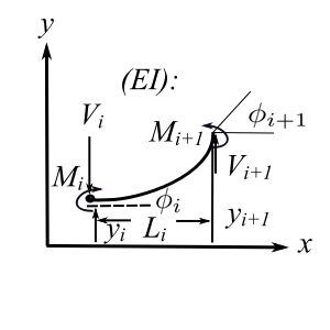
The state vector at position  is
is
![\[ \begin{Bmatrix} z \end{Bmatrix}_i = \begin{Bmatrix} y \\ \phi \\ M \\ V \end{Bmatrix} \]](https://engcourses-uofa.ca/wp-content/ql-cache/quicklatex.com-741407f123500d2ed10197d0843b069d_l3.png "Rendered by QuickLaTeX.com")
![\[ \begin{split} +\uparrow \Sigma F_y &= 0 \\ &= V_{i+1} - V_i \end{split} \]](https://engcourses-uofa.ca/wp-content/ql-cache/quicklatex.com-b3955c007786b14a3cabad6919486864_l3.png "Rendered by QuickLaTeX.com")
Therefore 
![\[ \begin{split} + \circlearrowleft \Sigma M_i &= -M_i + M_{i+1} + V_iL_i \\ M_{i+1} &= M_i - v_iL_i \end{split} \]](https://engcourses-uofa.ca/wp-content/ql-cache/quicklatex.com-f652f8cab0664e79149bd00d5d64a97e_l3.png "Rendered by QuickLaTeX.com")
Now must relate the slope and deflection at to 
| Deflection (L) | Angle (L) | |
 | | |
 | | |
![\[ \frac{ML^2}{2EI} \]](https://engcourses-uofa.ca/wp-content/ql-cache/quicklatex.com-d42893140d65f19fefc13ca4745ab305_l3.png "Rendered by QuickLaTeX.com")
![\[ \frac{ML}{EI} \]](https://engcourses-uofa.ca/wp-content/ql-cache/quicklatex.com-50ab0d398fef1e9976ce7317a088aa98_l3.png "Rendered by QuickLaTeX.com")
![\[ \frac{VL^3}{3EI} \]](https://engcourses-uofa.ca/wp-content/ql-cache/quicklatex.com-5b869345b06a22c30e11c05a6d56c4b1_l3.png "Rendered by QuickLaTeX.com")
![\[ \frac{VL^2}{2EI} \]](https://engcourses-uofa.ca/wp-content/ql-cache/quicklatex.com-95c05e8b519436d6d9678fce0ff57b4e_l3.png "Rendered by QuickLaTeX.com")
These are the so-called Myosotis Palustris formulae.
Therefore:
![\[ y_{i+1} = y_i + L_i\phi_i + \frac{M_{i+1}L^2_i}{2EI} + \frac{V_{i+1}L_i^3}{3EI} \]](https://engcourses-uofa.ca/wp-content/ql-cache/quicklatex.com-b22c2ec2af0ffad00e8c0d531a336d78_l3.png "Rendered by QuickLaTeX.com")
but
![\[ \begin{split} M_{i+1} &= M_i - V_iL_i \\ V_{i+1} &= V_i \end{split} \]](https://engcourses-uofa.ca/wp-content/ql-cache/quicklatex.com-37c88157a03c17783f9111f3c6097bb5_l3.png "Rendered by QuickLaTeX.com")
Therefore:
![\[ \begin{split} y_{i+1} &= y_i + L_i\phi_i + \frac{M_iL^2_i}{2EI} - \frac{V_iL_i^3}{2EI} + \frac{V_{i+1}L_i^3}{3EI} \\ y_{i+1} &= y_i + L_i\phi_i + \frac{M_j}{2}\Big(\frac{L^2}{EI}\Big)_i - \frac{V_i}{6}\Big(\frac{L^3}{EI}\Big)_i \end{split} \]](https://engcourses-uofa.ca/wp-content/ql-cache/quicklatex.com-48481eb913301b45967d11df3e6ad309_l3.png "Rendered by QuickLaTeX.com")
Also the slope
![\[ \begin{split} \phi_{i+1} &= \phi_i + M_{i+1}\Big(\frac{L}{EI}\Big)_i + \frac{V_{i+1}}{2}\Big(\frac{L^2}{EI}\Big)_i \\ \phi_{i+1} &= \phi_i + M_i \Big(\frac{L}{EI}\Big)_i - V_i\Big(\frac{L^2}{EI}\Big)_i + \frac{V_{i+1}}{2}\Big(\frac{L^2}{EI}\Big)_i \\ \phi_{i+1} &= \phi_i + M_i\Big(\frac{L}{EI}\Big)_i - \frac{V_i}{2}\Big(\frac{L^2}{EI}\Big)_i \end{split} \]](https://engcourses-uofa.ca/wp-content/ql-cache/quicklatex.com-b2bc01c1cdd694291d034d08cf4a638e_l3.png "Rendered by QuickLaTeX.com")
Therefore:
![\[ \begin{Bmatrix} z \end{Bmatrix}_{i+1} = \begin{bmatrix} 1 && L && \frac{L^2}{2EI} && -\frac{L^3}{6EI} \\ 0 && 1 && \frac{L}{EI} && -\frac{L^2}{2EI} \\ 0 && 0 && 1 && -L \\ 0 && 0 && 0 && 1 \end{bmatrix}_i \begin{Bmatrix} z \end{Bmatrix}_i \]](https://engcourses-uofa.ca/wp-content/ql-cache/quicklatex.com-b41532a88acfbbe59d61600463498f60_l3.png "Rendered by QuickLaTeX.com")
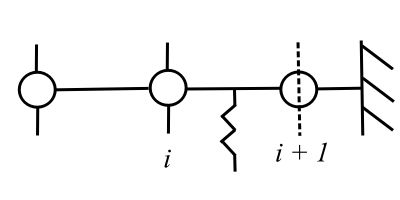
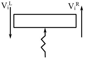
If we consider a point mass
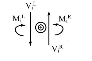
![\[ \uparrow \Sigma F_y = m \Ddot{x}_i = V_i^R - V_i^L \]](https://engcourses-uofa.ca/wp-content/ql-cache/quicklatex.com-30207bcdec246164755d442111a0e7a5_l3.png "Rendered by QuickLaTeX.com")
![\[ \begin{split} V_i^R &= V_i^L + m\Ddot{x}_i \\ &= V_i^L - mp^2x_i \end{split} \]](https://engcourses-uofa.ca/wp-content/ql-cache/quicklatex.com-75569bdf3d7acc74e39b23fb9fc8e37f_l3.png "Rendered by QuickLaTeX.com")
![\[ \begin{split} y_i^L &= y_i^R \\ \phi_i^L &= \phi_i^R \end{split} \]](https://engcourses-uofa.ca/wp-content/ql-cache/quicklatex.com-6300519c31b1732807b7f005f6fe7f35_l3.png "Rendered by QuickLaTeX.com")
![\[ \begin{Bmatrix} z \end{Bmatrix}_i^R = \begin{bmatrix} 1 && 0 && 0 && 0 \\ 0 && 1 && 0 && 0 \\ 0 && 0 && 1 && 0 \\ -mp^2 && 0 && 0 && 1 \end{bmatrix}_i \begin{Bmatrix} z \end{Bmatrix}_i^L \]](https://engcourses-uofa.ca/wp-content/ql-cache/quicklatex.com-41347ab777a21265b399b974e169841a_l3.png "Rendered by QuickLaTeX.com")
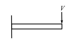
If we have a spring
![\[ \uparrow \Sigma F_y = V_i^R -y_ik_i - V_i^L \]](https://engcourses-uofa.ca/wp-content/ql-cache/quicklatex.com-0ca307ce27edabf06b820e8c10dbdb30_l3.png "Rendered by QuickLaTeX.com")
Therefore:
![\[ V_i^R = V_i^L + y_ik_i \]](https://engcourses-uofa.ca/wp-content/ql-cache/quicklatex.com-a78ea9094d6c5c91e9aa3499d995399b_l3.png "Rendered by QuickLaTeX.com")
![\[ \begin{Bmatrix} z \end{Bmatrix}_i^R = \begin{bmatrix} 1 && 0 && 0 && 0 \\ 0 && 1 && 0 && 0 \\ 0 && 0 && 1 && 0 \\ +k_i && 0 && 0 && 1 \end{bmatrix} \begin{Bmatrix} z \end{Bmatrix}_i^L \]](https://engcourses-uofa.ca/wp-content/ql-cache/quicklatex.com-b80e0bfe4dcd50de3dfbc6cb089471df_l3.png "Rendered by QuickLaTeX.com")
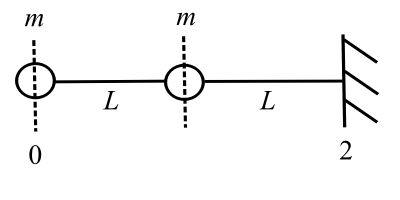
![\[ \begin{split} \hat{m} &= \frac{2m}{2L} \\ &= \frac{m}{L} \end{split} \]](https://engcourses-uofa.ca/wp-content/ql-cache/quicklatex.com-cad0a4f00fdb8881e2f5562dbb082131_l3.png "Rendered by QuickLaTeX.com")
![\[ \begin{Bmatrix} z \end{Bmatrix}_0 = \begin{Bmatrix} y_0 \\ \phi_0 \\ 0 \\ 0 \end{Bmatrix} \qquad \begin{Bmatrix} z \end{Bmatrix}_2 = \begin{Bmatrix} 0 \\ 0 \\ M_2 \\ V_2 \end{Bmatrix} \]](https://engcourses-uofa.ca/wp-content/ql-cache/quicklatex.com-3710a0483128e6079d219a8849b02e3d_l3.png "Rendered by QuickLaTeX.com")
![\[ \begin{Bmatrix} z \end{Bmatrix}_2^L = \begin{bmatrix} F \end{bmatrix}_{1-2} \begin{bmatrix} P \end{bmatrix}_1 \begin{bmatrix} F \end{bmatrix}_{0-1} \begin{bmatrix} P \end{bmatrix}_0 \begin{Bmatrix} z \end{Bmatrix}_0^L \]](https://engcourses-uofa.ca/wp-content/ql-cache/quicklatex.com-d092572188c5dc65d50b3b1ac42dc4e4_l3.png "Rendered by QuickLaTeX.com")
![\[ \begin{Bmatrix} 0 \\ 0 \\ M_2 \\ V_2 \end{Bmatrix} = \begin{bmatrix} u_{11} && u_{12} && u_{13} && u_{14} \\ u_{21} && u_{22} && u_{23} && u_{24} \\ u_{31} && u_{32} && u_{33} && u_{34} \\ u_{41} && u_{42} && u_{43} && u_{44} \end{bmatrix} \begin{Bmatrix} y \\ \phi \\ 0 \\ 0 \end{Bmatrix} \]](https://engcourses-uofa.ca/wp-content/ql-cache/quicklatex.com-504547dbb23a0fb194bc013d21037a23_l3.png "Rendered by QuickLaTeX.com")
Therefore:
![\[ \begin{split} u_{11} y_0 + u_{12} \phi_0 &= 0 \\ u_{21}y_0 + u_{22} \phi_0 &= 0 \end{split} \]](https://engcourses-uofa.ca/wp-content/ql-cache/quicklatex.com-dc896686492ae126cf3fa19e38ed22a2_l3.png "Rendered by QuickLaTeX.com")
Therefore:  is the equation of interest
Note that ![\big[F\big] \big[P\big]](https://engcourses-uofa.ca/wp-content/ql-cache/quicklatex.com-e08edca12c0fcd8b96b84e7d27667084_l3.png "Rendered by QuickLaTeX.com") is the same
is the same
Therefore:
![\[ \begin{split} \begin{bmatrix} F \end{bmatrix} \begin{bmatrix} P \end{bmatrix} &= \begin{bmatrix} 1 && L && \frac{L^2}{2EI} && -\frac{L^3}{6EI} \\ 0 && 1 && \frac{L}{EI} && -\frac{L^2}{2EI} \\ 0 && 0 && 1 && -L \\ 0 && 0 && 0 && 1 \end{bmatrix} \begin{bmatrix} 1 && 0 && 0 && 0 \\ 0 && 1 && 0 && 0 \\ 0 && 0 && 1 && 0 \\ -mp^2 && 0 && 0 && 1 \end{bmatrix} \\ &= \begin{bmatrix} 1+\frac{mp^2L^3}{6EI} && L && \frac{L^2}{2EI} && -\frac{L^3}{6EI} \\ +\frac{mp^2L^2}{2EI} && 1 && \frac{L}{EI} && -\frac{L^2}{2EI} \\ -mp^2L && 0 && 1 && -L \\ -mp^2 && 0 && 0 && 1 \end{bmatrix} \\ &= A \end{split} \]](https://engcourses-uofa.ca/wp-content/ql-cache/quicklatex.com-78798d514aafc80e4d28e271597cdf56_l3.png "Rendered by QuickLaTeX.com")
![\[ \begin{bmatrix} A \end{bmatrix}^2 = \begin{bmatrix} A \end{bmatrix} \begin{bmatrix} A \end{bmatrix} = \begin{bmatrix} U \end{bmatrix} \]](https://engcourses-uofa.ca/wp-content/ql-cache/quicklatex.com-f595ec136e2401b31de8e9750b326264_l3.png "Rendered by QuickLaTeX.com")
![\[ u_{ij} = \Sigma_k a_{ik}a_{kj} \]](https://engcourses-uofa.ca/wp-content/ql-cache/quicklatex.com-49ebac6a91f3788959b0d65c13cc3ed0_l3.png "Rendered by QuickLaTeX.com")
Therefore:
![\[ \begin{split} u_{11} &= a_{11}a_{11} + a_{12}a_{21} + a_{13}a_{31} + a_{14}a_{41} \\ &= \Big( 1 + \frac{mp^2L^3}{6EI}\Big)^2 + \frac{m^2L^3}{2EI} + \frac{mp^2L^3}{2EI} + \frac{mp^2L^3}{6EI} \\ &= 1 + \frac{9mp^2L^3}{6EI} + \Big( \frac{mp^2L^3}{6EI} \Big)^2 \\ &= 1 + 9\beta + \beta^2 \end{split} \]](https://engcourses-uofa.ca/wp-content/ql-cache/quicklatex.com-b09453a865cc3d784e9ac5d48f32053b_l3.png "Rendered by QuickLaTeX.com")
Where 
![\[ \begin{split} u_{22} &= a_{21}a_{12} + a_{22}a_{22} + a_{23}a_{32} + a_{24}a_{42} \\ &= \frac{mp^2L^3}{2EI} + 1 + 0 + 0 \\ &= 1 + 3\beta \end{split} \]](https://engcourses-uofa.ca/wp-content/ql-cache/quicklatex.com-1f078842cee551169ad9601485cdabb0_l3.png "Rendered by QuickLaTeX.com")
![\[ \begin{split} u_{12} &= a_{11}a_{12} + a_{12}a_{22} + a_{13}a_{32} + a_{14}a_{42} \\ &= L \Big( 1 + \frac{mp^2L^3}{6EI} \Big) + L \\ &= L(2 + \beta) \end{split} \]](https://engcourses-uofa.ca/wp-content/ql-cache/quicklatex.com-2a416fed98e38f04740abe132f98efa1_l3.png "Rendered by QuickLaTeX.com")
![\[ \begin{split} u_{21} &= a_{21}a_{11} + a_{22}a_{21} + a_{23}a_{31} + a_{24}a_{41} \\ &= \frac{mp^2L^2}{2EI}\Big( 1 + \frac{mp^2L^3}{6EI}\Big) + \frac{mp^2L^2}{2EI} + \frac{mp^2L^2}{EI} + \frac{mp^2L^2}{2EI} \\ &= \frac{5}{2}\frac{mp^2L^2}{EI} + \frac{1}{12}\Big( \frac{mp^2L^2}{EI} \Big)^2L \\ &= \frac{6\beta}{L}\Big( \frac{5}{2} + \frac{\beta}{2} \Big) \\ &= \frac{3\beta}{L}(5+\beta) \end{split} \]](https://engcourses-uofa.ca/wp-content/ql-cache/quicklatex.com-3ab1cdbe41dde73db8689e77aff9e466_l3.png "Rendered by QuickLaTeX.com")
![\[ \biggr[ 1 + \frac{9mp^2L^3}{6EI} + \Big(\frac{mp^2L^3}{6EI}\Big)^2 \biggr] \biggr[ 1 + \frac{m^2p^2L^3}{2EI} \biggr] - L \biggr[ 2 + \frac{mp^2L^3}{6EI} \biggr] \biggr[ \frac{5}{2} + \frac{1}{12} \frac{mp^2L^3}{EI} \biggr] \frac{mp^2L^2}{EI} = 0 \]](https://engcourses-uofa.ca/wp-content/ql-cache/quicklatex.com-58c6bd9c81545c25e929fa34dea7e939_l3.png "Rendered by QuickLaTeX.com")
let
![\[ \begin{split} \biggr[ 1 + 9\beta + \beta^2 \biggr] \biggr[ 1 + 3\beta \biggr] -6\beta \biggr[ \Big( 2 + \beta \Big) \Big( \frac{5}{2} + \frac{1}{2} \beta \Big) \biggr] &= 0 \\ \biggr[ 1 + 9\beta + \beta^2 \biggr] \biggr[ 1 + 3\beta \biggr] -3\beta \biggr[ \Big( 2 + \beta \Big) \Big( 5 + \beta \Big) \biggr] &= 0 \\ 1 + 9\beta + \beta^2 + 3\beta + 27\beta^2 + 3\beta^3 -3\beta \big[ 10 + 2\beta + 5\beta + \beta^2 \big] &= 0 \\ 1 + 12\beta +28\beta^2 + 3\beta^3 -30\beta -6\beta^2 - 15\beta^2 -3\beta^3 &= 0 \\ 7\beta^2 - 18\beta + 1 &= 0 \end{split} \]](https://engcourses-uofa.ca/wp-content/ql-cache/quicklatex.com-a9c718aeef9b8f28a12c82ad310ce4f0_l3.png "Rendered by QuickLaTeX.com")
![\[ \begin{split} \beta &= \frac{+18 \pm \sqrt{(18)^2-28}}{14} \\ &= \frac{18 \pm \sqrt{296}}{14} \\ &= \frac{9 \pm \sqrt{74}}{7} \end{split} \]](https://engcourses-uofa.ca/wp-content/ql-cache/quicklatex.com-8a8e9f7322ab572f3259a93df3f60dfc_l3.png "Rendered by QuickLaTeX.com")
![\[ \beta_{1,2} = 0.05681, \quad 2.5146 \]](https://engcourses-uofa.ca/wp-content/ql-cache/quicklatex.com-eb19e65e2e36a50f97b3065237953263_l3.png "Rendered by QuickLaTeX.com")
Therefore:
![\[ \begin{split} p_{1,2} &= \sqrt{\beta_{1,2}} \sqrt{6} \sqrt{\frac{EI}{mL^3}} \\ p_{1,2} &= 0.5838 \sqrt{\frac{EI}{mL^3}}, \quad 3.884 \sqrt{\frac{EI}{mL^3}} \end{split} \]](https://engcourses-uofa.ca/wp-content/ql-cache/quicklatex.com-67366e1dd61ef064bb1b376c7c36b654_l3.png "Rendered by QuickLaTeX.com")
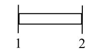
Compare with a beam
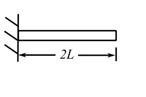
![\[ \begin{split} p_1 &= 3.52 \sqrt{\frac{EI}{\hat{m} (2L)^4}} \\ &= \frac{3.52}{4} \sqrt{\frac{EI}{\hat{m}L^4}} \\ &= 0.88 \sqrt{\frac{EI}{\hat{m}L^4}} \end{split} \]](https://engcourses-uofa.ca/wp-content/ql-cache/quicklatex.com-b4cd9b85507f50ef9bfbe528e1690401_l3.png "Rendered by QuickLaTeX.com")
Consider a Rayleigh approximation
![\[ p^2 \leq \frac{\int_0^L EI \big( \frac{d^2X}{dx^2} \big)^2 dx}{ \int_0^L m(X)^2 dx + \Sigma_{r=1}^k M \big\{ X(r,k)\big\}^2} \]](https://engcourses-uofa.ca/wp-content/ql-cache/quicklatex.com-0d052ded1fd7f31fdef516e637aa0220_l3.png "Rendered by QuickLaTeX.com")
assume 
![\[ \begin{split} p^2 &= \frac{\int_0^2 EI 4A^2 dx}{ m\big\{ AL^2\big\}^2 + m\big\{A4L^2\big\}^2 } \\ p^2 &= \frac{ 4A^2 EI(2L)}{ m\big\{ AL^2\big\}^2 + m\big\{A4L^2\big\}^2 } \\ &= \frac{8EIL}{17mL^4} \\ &= \frac{8EI}{17mL^3} \end{split} \]](https://engcourses-uofa.ca/wp-content/ql-cache/quicklatex.com-43a21dd130599507523da87d69b898bb_l3.png "Rendered by QuickLaTeX.com")
![\[ p \leq 0.686 \sqrt{\frac{EI}{mL^3}} \]](https://engcourses-uofa.ca/wp-content/ql-cache/quicklatex.com-812e17f665699e80c8d1d3e6fb5332a1_l3.png "Rendered by QuickLaTeX.com")
For forced steady state, assume all masses at 
picture
Therefore acceleration is 
![\[\{\mathfrak z\}_0 = \begin{Bmatrix}0 \\ F \end{Bmatrix}_0\]](https://engcourses-uofa.ca/wp-content/ql-cache/quicklatex.com-7537fc983cc69a1ea1ccecb47a0cdc4c_l3.png "Rendered by QuickLaTeX.com")
![\[\{\mathfrak z\}_1^L = \begin{bmatrix} 1 & \frac{1}{k} \\ 0 & 1 \end{bmatrix}\{\mathfrak z\}_0 \]](https://engcourses-uofa.ca/wp-content/ql-cache/quicklatex.com-55c7c1549dc88d206ddf7f76dfcfd8b4_l3.png "Rendered by QuickLaTeX.com")
![\[\{\mathfrak z\}_1^R = \begin{bmatrix} 1 & 0 \\ -m\omega^2 & 1 \end{bmatrix}\{\mathfrak z\}_1^L\]](https://engcourses-uofa.ca/wp-content/ql-cache/quicklatex.com-9df9705f6981c5a38c7bac9539fc3dc5_l3.png "Rendered by QuickLaTeX.com")
![\[\begin{split}\begin{Bmatrix} X \\ F_0 \end{Bmatrix} &= \{\mathfrak z\}_1^R \\&= \begin{bmatrix} 1 & 0 \\ -m\omega^2 & 1 \end{bmatrix} \begin{bmatrix} 1 & \frac{1}{k} \\ 0 & 1 \end{bmatrix} \begin{Bmatrix} 0 \\ F \end{Bmatrix} \\&= \begin{bmatrix} 1&\frac{1}{k} \\ -m\omega^2 & -\frac{m\omega^2}{k} + 1\end{bmatrix}\begin{Bmatrix} 0 \\ F \end{Bmatrix} \\&= \begin{Bmatrix}\frac{F}{k} \\ F\bigg(1-\frac{m\omega^2}{k}\bigg) \end{Bmatrix}\end{split}\]](https://engcourses-uofa.ca/wp-content/ql-cache/quicklatex.com-014a4f7e43b4c5fa3785cafdf2d6d582_l3.png "Rendered by QuickLaTeX.com")
Therefore:
![\[X = \frac{F}{k}\]](https://engcourses-uofa.ca/wp-content/ql-cache/quicklatex.com-58ba059e4d908b295b01b2e9da3bb383_l3.png "Rendered by QuickLaTeX.com")
![\[F_0 = F\bigg(1-\frac{m\omega^2}{k}\bigg)\]](https://engcourses-uofa.ca/wp-content/ql-cache/quicklatex.com-f2af768151bb02bb09ba055a2a9f3b54_l3.png "Rendered by QuickLaTeX.com")
![\[\begin{split}F &= \frac{F_0}{1 - \frac{m\omega^2}{k}} \\&=Xk\end{split}\]](https://engcourses-uofa.ca/wp-content/ql-cache/quicklatex.com-24d83c23d64f506d098388f6fc8012c4_l3.png "Rendered by QuickLaTeX.com")
Therefore:
![\[X = \frac{\frac{F_0}{k}}{1 - \frac{m\omega^2}{k}}\]](https://engcourses-uofa.ca/wp-content/ql-cache/quicklatex.com-9162244cd0e77663e2e56d870f8b4d72_l3.png "Rendered by QuickLaTeX.com")
![\[\begin{split} Xk &= F \\&= \frac{F_0}{1 - \frac{m\omega^2}{k}} \end{split}\]](https://engcourses-uofa.ca/wp-content/ql-cache/quicklatex.com-564211ee8ccf74d6deacdcb301329ecd_l3.png "Rendered by QuickLaTeX.com")
picture
![\[\{\mathfrak z\}_0 = \begin{Bmatrix} 0 \\ F \end{Bmatrix}_0\]](https://engcourses-uofa.ca/wp-content/ql-cache/quicklatex.com-00c5cd8161098db462caabfda400a677_l3.png "Rendered by QuickLaTeX.com")
![\[\mathfrak z_1^L = \begin{bmatrix} 1 & \frac{1}{2k} \\ 0 & 1 \end{bmatrix}\{\mathfrak z\}_0\]](https://engcourses-uofa.ca/wp-content/ql-cache/quicklatex.com-3917d76173929e6a29c64f9042ab28ae_l3.png "Rendered by QuickLaTeX.com")
picture
![\[x_1^L = x_1^R\]](https://engcourses-uofa.ca/wp-content/ql-cache/quicklatex.com-4c0e14a93d45d14b76e20c9096727ec5_l3.png "Rendered by QuickLaTeX.com")
![\[F_1^R -F_1^L = -m_1\omega^2x_1^L\]](https://engcourses-uofa.ca/wp-content/ql-cache/quicklatex.com-5d6efef02a3f1ae0f6b29fd846455925_l3.png "Rendered by QuickLaTeX.com")
Therefore:
![\[\begin{Bmatrix} x \\ F\end{Bmatrix}_1^R = \begin{bmatrix} 1 & 0 \\ -2m\omega^2 & 1 \end{bmatrix} \begin{Bmatrix} x \\ F \end{Bmatrix}_1^L \]](https://engcourses-uofa.ca/wp-content/ql-cache/quicklatex.com-7d8564c2af8054a53ce7cdaa01958e20_l3.png "Rendered by QuickLaTeX.com")
![\[\begin{Bmatrix} x \\ F\end{Bmatrix}_2^L = \begin{bmatrix} 1 & \frac{1}{k} \\ 0 & 1 \end{bmatrix} \begin{Bmatrix} x \\ F \end{Bmatrix}_1^R \]](https://engcourses-uofa.ca/wp-content/ql-cache/quicklatex.com-245f19e48064048a4e08803208078631_l3.png "Rendered by QuickLaTeX.com")
![\[\begin{split}\begin{Bmatrix} x_2 \\ F_0 \end{Bmatrix} &= \begin{Bmatrix} x \\ F\end{Bmatrix}_2^R \\&= \begin{bmatrix} 1 & 0 \\ -m\omega^2 & 1 \end{bmatrix} \begin{Bmatrix} x \\ F \end{Bmatrix}_2^L\end{split} \]](https://engcourses-uofa.ca/wp-content/ql-cache/quicklatex.com-8066c4262d4f48bc16244700e4e84962_l3.png "Rendered by QuickLaTeX.com")
Therefore:
![\[\begin{split}\begin{Bmatrix} x_2 \\ F_0 \end{Bmatrix}_2^R &= \begin{bmatrix} 1 & 0 \\ -m\omega^2 & 1 \end{bmatrix}\begin{bmatrix} 1 & \frac{1}{k} \\ 0 & 1\end{bmatrix} \begin{bmatrix} 1 & 0 \\ -2m\omega^2 & 1 \end{bmatrix}\begin{bmatrix} 1 & \frac{1}{2k} \\ 0 & 1 \end{bmatrix}\begin{Bmatrix} 0 \\ F \end{Bmatrix} \\&= \begin{bmatrix} 1 & \frac{1}{k}\\ -m\omega^2 & 1 - \frac{m\omega^2}{k}\end{bmatrix}\begin{bmatrix} 1 & \frac{1}{2k} \\ -2m\omega^2 & 1 - \frac{m\omega^2}{k}\end{bmatrix}\begin{Bmatrix} 0 \\ F \end{Bmatrix}\end{split}\]](https://engcourses-uofa.ca/wp-content/ql-cache/quicklatex.com-b3ad2be8b6747e8f58c24110d96b3691_l3.png "Rendered by QuickLaTeX.com")
![\[ \begin{Bmatrix} x_2 \\ F_0 \end{Bmatrix} = \begin{bmatrix} 1 - \frac{2m\omega^2}{k} & \frac{1}{2k} + \frac{1}{k}(1-\frac{m\omega^2}{k}) \\ -m\omega^2 - 2m\omega^2(1-\frac{m\omega^2}{k}) & -\frac{m\omega^2}{2k} + (1-\frac{m\omega^2}{k})^2\end{bmatrix}\begin{Bmatrix} 0 \\F \end{Bmatrix}\]](https://engcourses-uofa.ca/wp-content/ql-cache/quicklatex.com-795d898b3978e4cbcf70b21c26bc20ea_l3.png "Rendered by QuickLaTeX.com")
Therefore:
![\[x_2 = F\bigg(\frac{1}{2k} + \frac{1}{k}\bigg(1-\frac{m\omega^2}{k}\bigg)\bigg)\]](https://engcourses-uofa.ca/wp-content/ql-cache/quicklatex.com-a7c369d561d1823174046c0cf9a5b9bb_l3.png "Rendered by QuickLaTeX.com")
![\[F_0 = F\bigg(-\frac{m\omega^2}{2k} + \bigg(1-\frac{m\omega^2}{k}\bigg)^2\bigg)\]](https://engcourses-uofa.ca/wp-content/ql-cache/quicklatex.com-721b44ced77686f40d0b1a9bf5196c78_l3.png "Rendered by QuickLaTeX.com")
![\[x_2 = \frac{F}{k}\bigg[\frac{3}{2} - \frac{m\omega^2}{k}\bigg]\]](https://engcourses-uofa.ca/wp-content/ql-cache/quicklatex.com-6fa3c41c3c92704b6f06ef16670af00d_l3.png "Rendered by QuickLaTeX.com")
![\[F = \frac{F_0}{-\frac{m\omega^2}{2k} + 1 - \frac{2m\omega^2}{k} + (\frac{m\omega^2}{k})^2}\]](https://engcourses-uofa.ca/wp-content/ql-cache/quicklatex.com-3a8f04ee1f9e8410b877cfe1929e30e0_l3.png "Rendered by QuickLaTeX.com")
Therefore:
![\[\begin{split}x_2 &=\frac{ \frac{F_0}{k}(\frac{3}{2}- \frac{m\omega^2}{k})}{1 - \frac{5m\omega^2}{2k} + (\frac{m\omega^2}{k})^2} \\&=\frac{ \frac{F_0}{k}(\frac{3}{2}- \frac{m\omega^2}{k})}{(1-\frac{m\omega^2}{2k})(1-\frac{2m\omega^2}{k})}\end{split}\]](https://engcourses-uofa.ca/wp-content/ql-cache/quicklatex.com-43b9616aac78a77d6d50b43e693383e9_l3.png "Rendered by QuickLaTeX.com")
When  :
:
![\[x_1 = \frac{\frac{F_0}{2k}}{(1-\frac{m\omega^2}{2k})(1-\frac{2m\omega^2}{k})}\]](https://engcourses-uofa.ca/wp-content/ql-cache/quicklatex.com-318f4dadd9a70ebbb71f3018c3b29391_l3.png "Rendered by QuickLaTeX.com")
This approach to formulation and solution to vibration problems is generally called the impedance approach and is commonly used in electrical current systems. It can be further expanded to include damping. The approach is identical except that the matrices are complex as this allows the phase relations to be handled. (In the undamped case displacement/forces are either in phase or 180˚ out of phase).