
Review of single and multi-degree of freedom (mdof) systems: Stiffness and Flexibility Influence Coefficients
We can use the Newtonian approach to find the stiffness matrix and equations of motion. However, we can also use influence coefficients for both the mass and stiffness matrices.
Consider the definition of stiffness and flexibility influence coefficients:
S.I.C
 is the force (moment) required at coordinate
  to maintain a unit linear (angular) displacement at coordinate
  with all other coordinates held fixed at zero
F.I.C
 is the linear (angular) displacement at coordinate due to a unit force (moment) applied at coordinate with all other coordinates free to move.
NOTE: All forces (moments) and displacements (rotations) are taken to be applied in the positive direction. The sign of the resulting forces (moments) or displacements (rotations) are determined to be positive or negative.
Also note that:
![\[ [a_{ij}]^{-1} = [k_{ij}] \]](https://engcourses-uofa.ca/wp-content/ql-cache/quicklatex.com-03bc065570ba213fa0f0e088a1ac5121_l3.png "Rendered by QuickLaTeX.com")
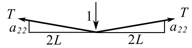
Example
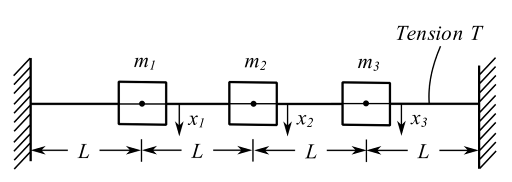
Stiffness
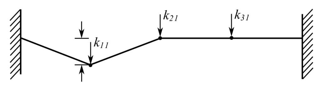
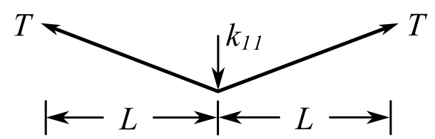
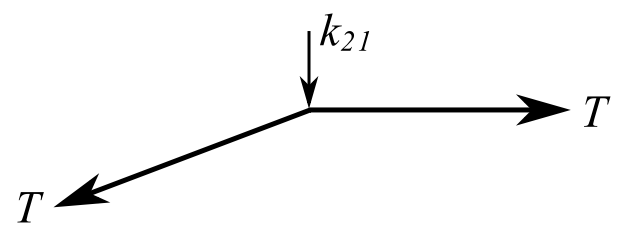
Therefore:
![\[k_{11} = \frac{2T}{L},\ k_{21} = \frac{-T}{L},\ k_{31} = 0 \]](https://engcourses-uofa.ca/wp-content/ql-cache/quicklatex.com-e123ba93c5ca63f7042a495668db0a3b_l3.png "Rendered by QuickLaTeX.com")
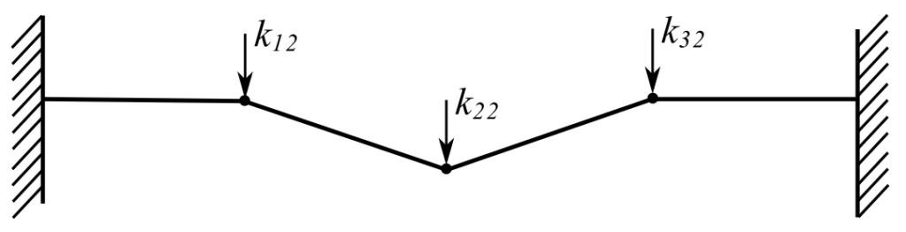
![\[k_{22} = \frac{2T}{L},\ k_{12} = k_{32} = \frac{-T}{L} \]](https://engcourses-uofa.ca/wp-content/ql-cache/quicklatex.com-6d1d456890b5d4c084ceb6c0d7dfc300_l3.png "Rendered by QuickLaTeX.com")
Therefore:
![\[ \frac{T}{L} \begin{bmatrix} 2 & -1 & 0 \\ -1 & 2 & -1 \\ 0 & -1 & 2 \end{bmatrix} = [k] \]](https://engcourses-uofa.ca/wp-content/ql-cache/quicklatex.com-3ed7ec2da177632b4e386733e5b0770f_l3.png "Rendered by QuickLaTeX.com")
Flexibilty
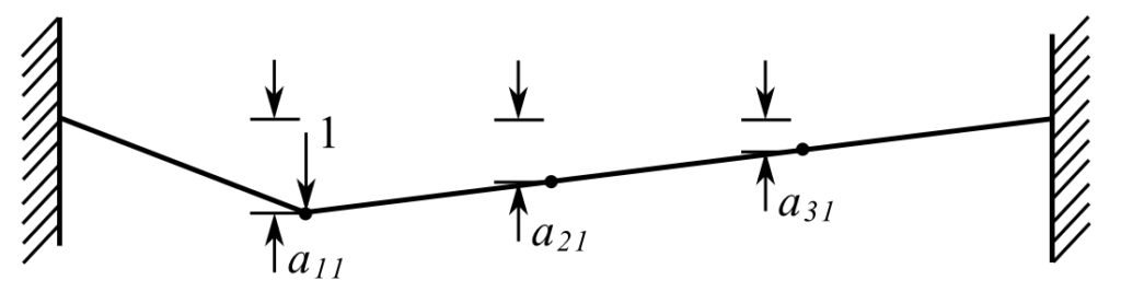
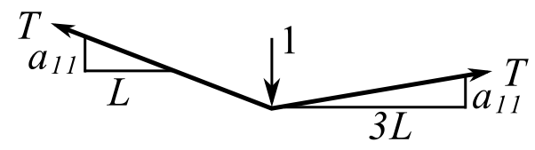
![\[ T\Big[\frac{a_{11}}{L} + \frac{a_{11}}{3L}\Big] = 1 \]](https://engcourses-uofa.ca/wp-content/ql-cache/quicklatex.com-8bdb126e1a07ad896f0c6501fe71ad63_l3.png "Rendered by QuickLaTeX.com")
![\[ T\Big[\frac{4a_{11}}{3L}\Big] = 1\]](https://engcourses-uofa.ca/wp-content/ql-cache/quicklatex.com-c9bed2ccf49a1abcdce0aa17e75bc828_l3.png "Rendered by QuickLaTeX.com")
![\[a_{11} = \frac{3L}{4T} = a_{33}\]](https://engcourses-uofa.ca/wp-content/ql-cache/quicklatex.com-0a7ae472fca5f5a72e38df4ff098cea4_l3.png "Rendered by QuickLaTeX.com")
![\[a_{21} = \frac{2}{3}a_{11} = \frac{L}{2T} \]](https://engcourses-uofa.ca/wp-content/ql-cache/quicklatex.com-ca9c614eda416e9253b20b2aeca4aa8e_l3.png "Rendered by QuickLaTeX.com")
![\[a_{31} = \frac{1}{3}a_{11} = \frac{L}{4T} \]](https://engcourses-uofa.ca/wp-content/ql-cache/quicklatex.com-d0fe2ec087e8753263cabfc17d29a583_l3.png "Rendered by QuickLaTeX.com")
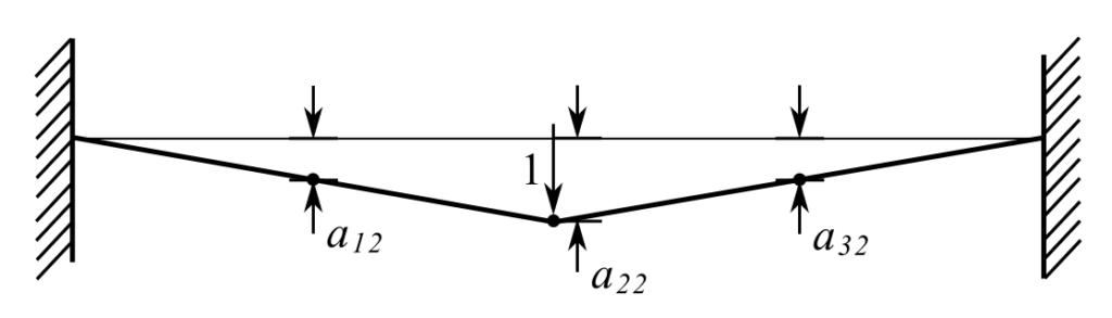
![\[1 = 2T\frac{a_{22}}{2L}\]](https://engcourses-uofa.ca/wp-content/ql-cache/quicklatex.com-63f1b495cc60cd7560acd19d64226751_l3.png "Rendered by QuickLaTeX.com")
Therefore:
![\[1 = T\frac{a_{22}}{L}\]](https://engcourses-uofa.ca/wp-content/ql-cache/quicklatex.com-3e1024368bef591367754b5e5e837a18_l3.png "Rendered by QuickLaTeX.com")
![\[a_{22} = \frac{L}{T}\]](https://engcourses-uofa.ca/wp-content/ql-cache/quicklatex.com-191b869d57436ee5c446060c78449a87_l3.png "Rendered by QuickLaTeX.com")
![\[a_{12} = \frac{L}{2T} = a_{32}\]](https://engcourses-uofa.ca/wp-content/ql-cache/quicklatex.com-b29afbaa8e84be7f8e62e14a9814504b_l3.png "Rendered by QuickLaTeX.com")
Thus:
![\[\frac{L}{T}\begin{bmatrix} \frac{3}{4} & \frac{1}{2} & \frac{1}{4} \\[2ex] \frac{1}{2} & 1 & \frac{1}{2} \\[2ex] \frac{1}{4} & \frac{1}{2} & \frac{3}{4} \end{bmatrix} = [a_{ij}] \]](https://engcourses-uofa.ca/wp-content/ql-cache/quicklatex.com-1fed315c687f2986ccd5fd6d802e4dff_l3.png "Rendered by QuickLaTeX.com")
Therefore:
![\[ \begin{split} [a][k] &= \begin{bmatrix} \frac{3}{4} & \frac{1}{2} & \frac{1}{4} \\[2ex] \frac{1}{2} & 1 & \frac{1}{2} \\[2ex] \frac{1}{4} & \frac{1}{2} & \frac{3}{4} \end{bmatrix} \begin{bmatrix} 2 & -1 & 0 \\ -1 & 2 & -1 \\ 0 & -1 & 2 \end{bmatrix} \\&= \begin{bmatrix} \frac{3}{2} - \frac{1}{2} & -\frac{3}{4} + 1 -\frac{1}{4} & -\frac{1}{2} + \frac{1}{2} \\[2ex] 1-1 & -\frac{1}{2} + 2 - \frac{1}{2} & -1+1 \\[2ex] \frac{1}{2} - \frac{1}{2} & -\frac{1}{4} + 1 - \frac{3}{4} & -\frac{1}{2} + \frac{3}{2} \end{bmatrix} \\&= \begin{bmatrix} 1 & 0 & 0 \\ 0 & 1 & 0 \\ 0 & 0 & 1 \end{bmatrix} \end{split}\]](https://engcourses-uofa.ca/wp-content/ql-cache/quicklatex.com-39cf4038fe2ec4611e83b9566817a597_l3.png "Rendered by QuickLaTeX.com")
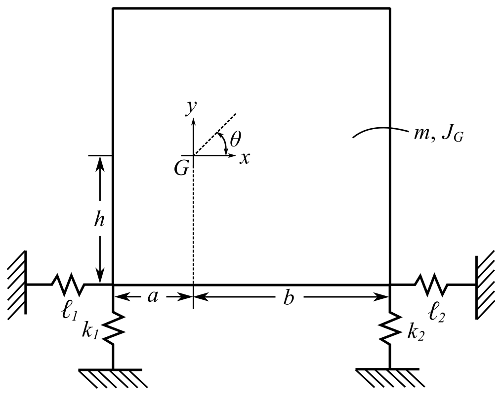
As an example of MDOF, consider a general planar situation which can be specialized to different industrial situations. Many of these problems can be initially modelled as SDOF ones, and then MDOF analysis will allow interpretations of the simplifying assumptions made.
NOTE: While the body shown is a rectangular shape, it can be any rigid body with a mass  and moment of inertia
  about an axis
  to the plane through the center of gravity. The horizontal stiffness components, designated by
  are most often just the lateral stiffness of the vertically mounted spring. For real springs, the lateral spring stiffness may be hard to find in the literature. For coil springs, it is often in the range of
  times the longitudinal value.
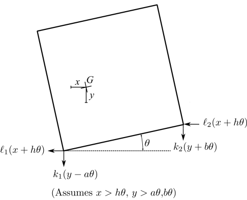
![\[\begin{split} +\rightarrow \sum F_x &= m\ddot{x} \\&= -\ell_1(x + h\theta) - \ell_2(x+h\theta) \quad (1) \end{split} \]](https://engcourses-uofa.ca/wp-content/ql-cache/quicklatex.com-036b3c6b79a985f435addcfc2120bb35_l3.png "Rendered by QuickLaTeX.com")
![\[\begin{split} +\uparrow \sum F_y &= m\ddot{y} \\&= -k_1(y-a\theta) - k_2(y + b\theta) \quad (2) \end{split} \]](https://engcourses-uofa.ca/wp-content/ql-cache/quicklatex.com-4cf83e1a05a9b849ed701b44f4384ba6_l3.png "Rendered by QuickLaTeX.com")
![\[+\circlearrowleft \sum M_G = J_G\ddot{\theta} = -\ell_1(x+h\theta)h - \ell_2(x+h\theta)h + k_1(y-a\theta)a - k_2(y + b\theta)b \quad (3) \]](https://engcourses-uofa.ca/wp-content/ql-cache/quicklatex.com-d19dc6c1d9192b88adc52bb2d67aad6f_l3.png "Rendered by QuickLaTeX.com")
![\[m\ddot{x} + \ell_1x + \ell_1h\theta + \ell_2x + \ell_2h\theta = 0 \quad (1)\]](https://engcourses-uofa.ca/wp-content/ql-cache/quicklatex.com-55fa4bad2b74d3aa300261816aaadcfd_l3.png "Rendered by QuickLaTeX.com")
![\[m\ddot{y} + k_1y - k_1a\theta + k_2y + k_2b\theta = 0 \quad (2) \]](https://engcourses-uofa.ca/wp-content/ql-cache/quicklatex.com-be27fc60b2015749f66af6d0f3be08c7_l3.png "Rendered by QuickLaTeX.com")
![\[J_G\ddot{\theta} + \ell_1xh + \ell_1h^2\theta + \ell_2xh + \ell_2h^2\theta - k_1ay + k_1a^2\theta + k_2by + k_2b^2\theta = 0 \quad (3) \]](https://engcourses-uofa.ca/wp-content/ql-cache/quicklatex.com-d43266f1fd8669884dbfbfedd44935e1_l3.png "Rendered by QuickLaTeX.com")
In matrix form:
![\[ \begin{Bmatrix} 0 \\ 0 \\ 0 \end{Bmatrix} = \begin{bmatrix} m & 0 & 0 \\ 0 & m & 0 \\ 0 & 0 & J_G \end{bmatrix} \begin{Bmatrix} \ddot{x} \\ \ddot{y} \\ \ddot{\theta} \end{Bmatrix} + \begin{bmatrix} \ell_1 + \ell_2 & 0 & (\ell_1+\ell_2)h \\ 0 & k_1 + k_2 & k_2b - k_1a \\ (\ell_1+\ell_2)h & k_2b-k_1a & h^2(\ell_1+\ell_2) + k_1a^2 +k_2b^2 \end{bmatrix} \begin{Bmatrix} x \\ y \\ z \end{Bmatrix} \]](https://engcourses-uofa.ca/wp-content/ql-cache/quicklatex.com-e39117a0babc44b7d93bf1909ecd4a3e_l3.png "Rendered by QuickLaTeX.com")
Now find the stiffness matrix using influence coefficients.
First consider a unit displacement in the  direction only:
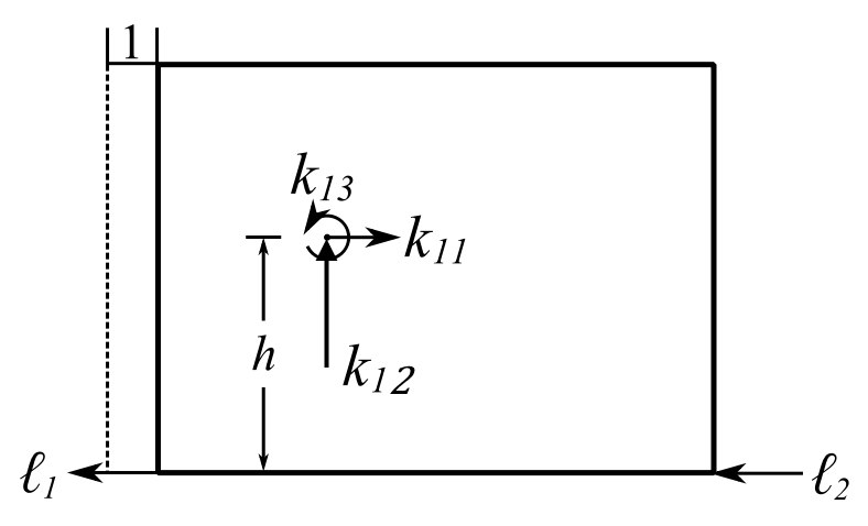
![\[\begin{split} + \rightarrow\sum F_x &= 0 \\& = k_{11} - (\ell_1 + \ell_2) \\ \implies k_{11} &= \ell_1 + \ell_2\end{split}\]](https://engcourses-uofa.ca/wp-content/ql-cache/quicklatex.com-6e2f7f9e42e265826d8527d0ca96681f_l3.png "Rendered by QuickLaTeX.com")
![\[\begin{split} + \uparrow\sum F_y &= 0 \\ \implies k_{12} &= 0 \end{split}\]](https://engcourses-uofa.ca/wp-content/ql-cache/quicklatex.com-31b5c6f86fd42a2d67e9c179b341ee50_l3.png "Rendered by QuickLaTeX.com")
![\[\begin{split} +\circlearrowleft\sum M_G &= 0 \\& = k_{13} - (\ell_1+\ell_2)h\\ \implies k_{13} &=(\ell_1 + \ell_2)h \end{split} \]](https://engcourses-uofa.ca/wp-content/ql-cache/quicklatex.com-779af71f92de894340901d87d7bca019_l3.png "Rendered by QuickLaTeX.com")
For the  direction unit displacement:
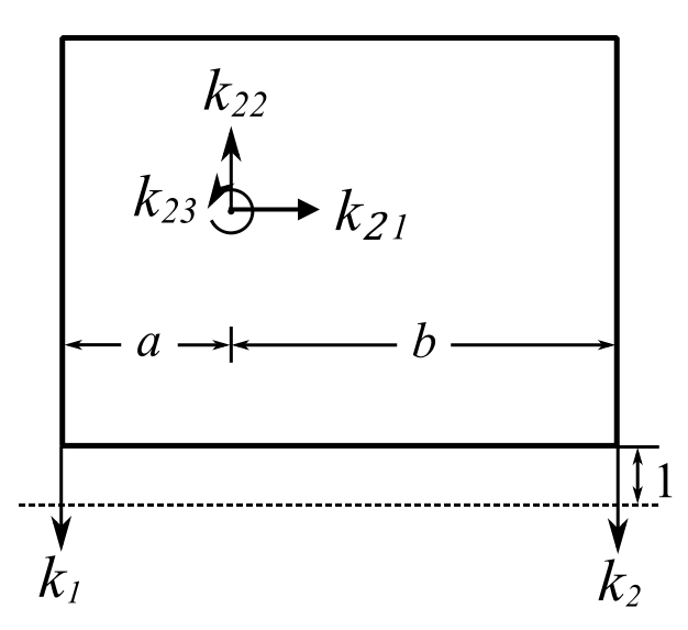
![\[ \begin{split} +\uparrow\sum F_y & = 0 \\& = k_{22} - (k_1 + k_2) \end{split} \]](https://engcourses-uofa.ca/wp-content/ql-cache/quicklatex.com-57e7b1432ea1d9beabd88cb2e2432eea_l3.png "Rendered by QuickLaTeX.com")
![\[\implies k_{22} = k_1 + k_2 \]](https://engcourses-uofa.ca/wp-content/ql-cache/quicklatex.com-18e43b35b4c61d02e5823b37c153d368_l3.png "Rendered by QuickLaTeX.com")
![\[\begin{split} + \circlearrowleft \sum M_G &= 0 \\& = k_{23} + k_1a - k_2b \end{split}\]](https://engcourses-uofa.ca/wp-content/ql-cache/quicklatex.com-67ebbd477c81aa31e57199071551da80_l3.png "Rendered by QuickLaTeX.com")
![\[\implies k_{23} = k_2b-k_1a\]](https://engcourses-uofa.ca/wp-content/ql-cache/quicklatex.com-65cd3cbb587236ea2e6a2ab15908ba1c_l3.png "Rendered by QuickLaTeX.com")
![\[+\rightarrow \sum F_x = 0\]](https://engcourses-uofa.ca/wp-content/ql-cache/quicklatex.com-04da62e6d51d65bf7492f3a180583472_l3.png "Rendered by QuickLaTeX.com")
![\[\implies k_{21} = 0\]](https://engcourses-uofa.ca/wp-content/ql-cache/quicklatex.com-bf04848d530c20390010b7686a528612_l3.png "Rendered by QuickLaTeX.com")
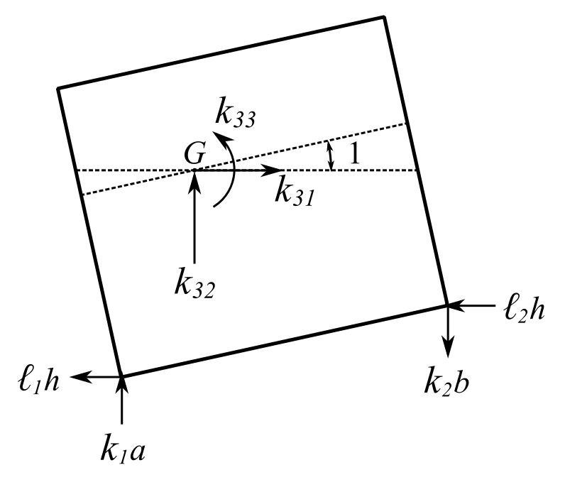
Assuming all summations for direction, direction and moment equal to  :
:
![\[+\rightarrow \sum F_x = k_{31} - \ell_1h - \ell_2h = 0\]](https://engcourses-uofa.ca/wp-content/ql-cache/quicklatex.com-164ffcc9238eaf390c9268b76dd273d0_l3.png "Rendered by QuickLaTeX.com")
![\[\implies k_{31} = (\ell_1 + \ell_2)h \]](https://engcourses-uofa.ca/wp-content/ql-cache/quicklatex.com-f416984d416305b3cad5ca5d34d191ca_l3.png "Rendered by QuickLaTeX.com")
![\[+\uparrow \sum F_y = k_{32} + k_1a-k_2b = 0\]](https://engcourses-uofa.ca/wp-content/ql-cache/quicklatex.com-9629dfc2d2f12edfa98d50efa3e4844b_l3.png "Rendered by QuickLaTeX.com")
![\[ \implies k_{32} = k_2b - k_1a\]](https://engcourses-uofa.ca/wp-content/ql-cache/quicklatex.com-aed796f3714a7e6a9390ae1e93a67cb5_l3.png "Rendered by QuickLaTeX.com")
![\[+\circlearrowleft \sum M_G = k_{33} -(\ell_1 + \ell_2)h^2 - k_1a^2 - k_2b^2 = 0\]](https://engcourses-uofa.ca/wp-content/ql-cache/quicklatex.com-0671417040122f840a7a0f063a97c124_l3.png "Rendered by QuickLaTeX.com")
Therefore:
![\[k_{33} = (\ell_1+\ell_2)h^2 + k_1a^2 + k_2b^2\]](https://engcourses-uofa.ca/wp-content/ql-cache/quicklatex.com-4410aa7c8ef4f2b6d5f9b6477dd739fa_l3.png "Rendered by QuickLaTeX.com")
This yields the same stiffness matrix.
As long as we use the motions about the center of gravity then the inertia (mass) matrix is just the mass or the mass moment of inertia about the center of gravity. If we use coordinates to describe the motion that are not related to the absolute motion of the center of gravity then the stiffness matrix may not be symmetric and the mass matrix will not be diagonal.
Inertia Influence Coefficients
The elements of the mass matrix,  can be determined through the use of inertia influence coefficients. They are defined as the set of impulses applied at the points (representing the coordinate directions)
  respectively to produce a unit velocity at point and zero velocity at every other point.
NOTE: If  denotes an angular coordinate then
  represents an angular velocity
Thus for a multi-degree of freedom system, the total impulses at points is:
![\[\tilde{F}_i = \sum_{j = 1}^n m_{ij}\dot{x}_j\]](https://engcourses-uofa.ca/wp-content/ql-cache/quicklatex.com-36a3c1dbf3a07aeb107043a0f4fb8c08_l3.png "Rendered by QuickLaTeX.com")
![\[\{\tilde{F}\} = [m]\{\dot{x}_i\}\]](https://engcourses-uofa.ca/wp-content/ql-cache/quicklatex.com-6933882c95d8d58d6a19f74e6f034366_l3.png "Rendered by QuickLaTeX.com")
![\[[m] = \begin{bmatrix} m_{11} & \ldots &m_{1n} \\ \vdots & & \vdots \\ m_{n1} & \ldots & m_{nn} \end{bmatrix}\]](https://engcourses-uofa.ca/wp-content/ql-cache/quicklatex.com-07e5db66e0ffa10883138e1113cb82fb_l3.png "Rendered by QuickLaTeX.com")
![\[\tilde{F} = \begin{Bmatrix} F_1 \\ \vdots \\ F_n \end{Bmatrix} \]](https://engcourses-uofa.ca/wp-content/ql-cache/quicklatex.com-8d146a6d56125c24abab7e4670b12145_l3.png "Rendered by QuickLaTeX.com")
![\[\{\dot{x}\} = \begin{Bmatrix} \dot{x}_1 \\ \vdots \\ \dot{x}_n \end{Bmatrix} \]](https://engcourses-uofa.ca/wp-content/ql-cache/quicklatex.com-d0141507d6bf4193a9fabc87c4c6344e_l3.png "Rendered by QuickLaTeX.com")
To find the 
- Assume that a set of impulses
 are applied at all points
  as to produce a unit velocity at point only(with zero velocity in all the after directions (coordinates)). By definition the set of impulses
  denote the influence inertia coefficients
 - Repeat the procedure for each point
 .
.
Example
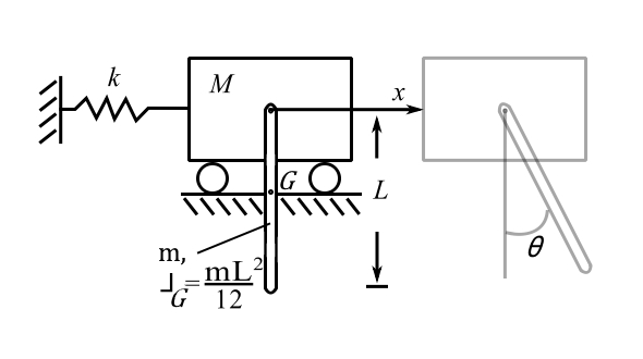
First apply unit velocity to only:
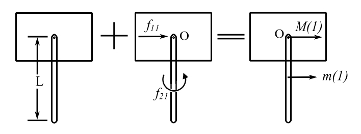
![\[ \begin{split} +\rightarrow \sum L &= f_{11} \\&= (M+m) \\&= m_{11} \end{split}\]](https://engcourses-uofa.ca/wp-content/ql-cache/quicklatex.com-8cbd2b0391beb7647976416643e703d2_l3.png "Rendered by QuickLaTeX.com")
![\[\begin{split} +\circlearrowleft \sum H_0 &= f_{21} \\&= m\frac{L}{2} \\& = m_{21}\end{split}\]](https://engcourses-uofa.ca/wp-content/ql-cache/quicklatex.com-1ac4c6b0ea9b6dbb4714d240ad408eea_l3.png "Rendered by QuickLaTeX.com")
Apply unit velocity(angular) to  only
only
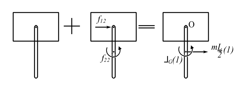
![\[\begin{split} +\rightarrow \sum L &= f_{12} \\&= \frac{mL}{2} \\&= m_{12}\end{split}\]](https://engcourses-uofa.ca/wp-content/ql-cache/quicklatex.com-b8ff2e6b4f5b59305c22c1d0549f9c96_l3.png "Rendered by QuickLaTeX.com")
![\[ \begin{split} +\circlearrowleft \sum H_0 &= J_G(1) + \frac{mL}{2}(1)\frac{L}{2} \\&= \frac{1}{12}mL^2+\frac{mL^2}{4} \\&= \frac{mL^2}{3} \\&=m_{22}\end{split} \]](https://engcourses-uofa.ca/wp-content/ql-cache/quicklatex.com-547c4f2a226238044df8e886a3342e3d_l3.png "Rendered by QuickLaTeX.com")
Therefore:
![\[\begin{bmatrix} M + m & \frac{mL}{2} \\ \frac{mL}{2} & \frac{mL^3}{3} \end{bmatrix}\]](https://engcourses-uofa.ca/wp-content/ql-cache/quicklatex.com-43a486491658baf5d7f4194b2859e483_l3.png "Rendered by QuickLaTeX.com")
Now find the stiffness matrix
Apply unit deflection to only:
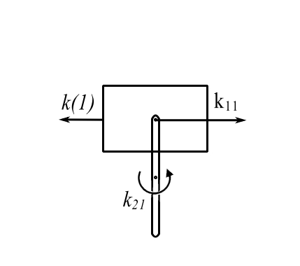
Therefore
![\[k_{11} = k\]](https://engcourses-uofa.ca/wp-content/ql-cache/quicklatex.com-ed339fe687ac9d0f731774af70fbbb0e_l3.png "Rendered by QuickLaTeX.com")
![\[k_{21} = 0\]](https://engcourses-uofa.ca/wp-content/ql-cache/quicklatex.com-48d7a861aa472cbc6844f8095dbcb7bd_l3.png "Rendered by QuickLaTeX.com")
Apply unit deflection to only:
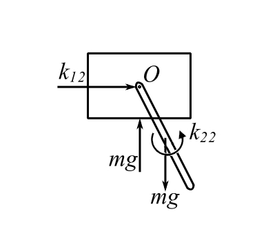
![\[ \begin{split} +\circlearrowleft \sum M_0 &= k_{22} - mg\frac{\ell}{2}(1) \\&= 0\end{split}\]](https://engcourses-uofa.ca/wp-content/ql-cache/quicklatex.com-695f7403c693b6dcf824c02ac8f8e0a5_l3.png "Rendered by QuickLaTeX.com")
![\[ k_{22} = mg\frac{\ell}{2}\]](https://engcourses-uofa.ca/wp-content/ql-cache/quicklatex.com-593ddfe3fe41d8480d84222e9e3b3dac_l3.png "Rendered by QuickLaTeX.com")
![\[ k_{12} = 0\]](https://engcourses-uofa.ca/wp-content/ql-cache/quicklatex.com-0ae33c785c54327ead2048f0b4b97d8f_l3.png "Rendered by QuickLaTeX.com")
Therefore:
![\[\begin{bmatrix} M + m & \frac{mL}{2} \\ \frac{mL}{2} & \frac{mL^3}{3} \end{bmatrix} \begin{Bmatrix} \ddot{x} \\ \ddot{\theta} \end{Bmatrix} + \begin{bmatrix} k_1 & 0 \\0 & \frac{mgL}{2} \end{bmatrix}\begin{Bmatrix} x \\\theta \end{Bmatrix}= \begin{Bmatrix} 0 \\0 \end{Bmatrix}\]](https://engcourses-uofa.ca/wp-content/ql-cache/quicklatex.com-ebed988f0f69b31da17571795870d424_l3.png "Rendered by QuickLaTeX.com")
It is explained in great details and so clear, I have found such information on springs coefficients calculation nowerewhere. So greatful