Engineering at Alberta Courses » Introduction and Review

Review of single and multi-degree of freedom (mdof) systems: Introduction and Review

We are interested in small motions about some equilibrium positions. For SDOF systems, $x$ is usually measured from this static equilibrium position.

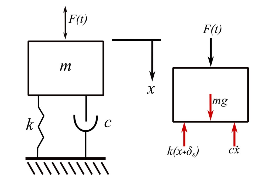
$\begin{split}+\downarrow \sum{F_x} &= m \ddot{x} \\&= -k(x+\delta_s)-c\dot{x} + F(t)+mg\end{split}$

Let $\dot{x}, \ddot{x} = 0$ for static equilibrium. Therefore:

$-k\delta_s+mg = 0$

Let $\delta_s = \frac{mg}{k}$ . Therefore:

$m\ddot{x}+c\dot{x} +kx = F(t)$

All SDOF systems can be reduced to this form (assuming viscous damping):

$m_e\ddot{x}+c_e\dot{x} +k_ex = F(t) \quad$

Where $e$ means equivalent. To determine the nature of the motion, first consider this linearized equation of free vibration (Note: May have to linearize).

Assume $x_H = Ae^{st}$ (homogeneous), where $A$ is constant and $s$ is to be determined.

$m_es^2 + c_es+k_e = 0$

$\begin{split}s_{1,2} &= -\frac{c_e}{2m_e} \pm \sqrt{\Big(\frac{c_e}{2m_e}\Big)^2-\frac{k_e}{m_e}}\\&= -\frac{\tilde{c}}{2} \pm \sqrt{\Big(\frac{\tilde{c}}{2}\Big)^2-\tilde{k}}\end{split}$

If $s_{1,2}$ are real and negative, then $x\rightarrow 0$ as $t \rightarrow\infty$ . If either of $s_1$ or $s_2$ are real and positive, then the solution increases with time.

If $s_{1,2}$ are complex, then they are complex conjugates and the nature of the motion depends on the real part. If the real part is negative, $x\rightarrow 0$ as $t\rightarrow \infty$ . If positive, $x\rightarrow \infty$ as $t \rightarrow \infty$ . If the real part is zero, the motion is oscillatory and this is the borderline case between stability and instability.

Consider all cases:

$\tilde{c} > 0 \quad \tilde{k} > 0$ . The roots have a negative real part and is stable regardless of $\tilde{k}$ . If $|\tilde{k}|$ is larger than $|\frac{\tilde{c}}{2}|^2$ , there will be an oscillatory part, but $x\rightarrow0$ as $t \rightarrow \infty$ . This is called asymptotically stable.
$\tilde{c} = 0 \quad \tilde{k}>0$ . The roots are imaginary, and the system is borderline stable.
$\tilde{k}<0 \quad\tilde{c}\le 0$ . The roots have a positive real part, or are complex conjugates. Therefore, the system is unstable.
$\tilde{k}<0 \quad\tilde{c}>0$ One root has a positive real part. Therefore the system is unstable. The damping cannot overcome the negative spring.
$\tilde{k}>0 \quad\tilde{c}<0$ . The roots have a positive real part, and therefore the system is unstable. Negative damping feeds energy into the system.

Consider the solution for free damped vibration:

$m_e \ddot{x}+c_e\dot{x} +k_e x=0$

Drop $e$ , but remember that $m$ , $c$ , $k$ are equivalent. Thus:

$\ddot{x}+\frac{c}{m}\dot{x}+\frac{k}{m}x = 0$

Again, assume that $x=Ae^{st}$ . Thus:

$s_{1,2}= \frac{-c}{2m}\pm\sqrt{\Big(\frac{c}{2m}\Big)^2-\frac{k}{m}}$

The critical value is then when:

$\Big(\frac{c_c}{2m}\Big)^2=\frac{k}{m} := p^2$

Alternatively:

$c_c = 2mp$

Define $\zeta := \frac{c}{c_c}$ . Then:

$\frac{c}{2m} = \frac{c}{c_c}\frac{2mp}{2m} = \zeta p$

Thus:

$s_{1,2} = \Big(-\zeta \pm \sqrt{\zeta ^2-1}\Big)p$

Where $\zeta$ is the damping ratio (system parameter).

Assuming $0<\zeta<1$ :

$x(t) = e^{-\zeta pt}\Big[C_1e^{i\sqrt{1-\zeta^2}}pt+C_2e^{-i\sqrt{1-\zeta^2}}pt\Big]$

And using $e^{\pm i\theta}=\cos{\theta}\pm i\sin{\theta}$ :

$x(t) = e^{-\zeta pt}\Big[A\cos{\sqrt{1-\zeta^2}pt+B\sin{\sqrt{1-\zeta^2}pt}}\Big]$

Using initial conditions $x(0) = x_0$ , $\dot{x}(0) = v_0$ , we get the following:

$x(t)=e^{-\zeta pt}\Big[x_0 \cos\sqrt{1-\zeta^2} pt + \frac{v_0 + \zeta p x_0}{p\sqrt{1-\zeta^2}}\sin{\sqrt{1-\zeta^2}pt}\Big]$

We can write this as:

$x(t) = e^{-\zeta pt}\Big[\sqrt{A^2+B^2}\sin{(\sqrt{1-\zeta^2}pt + \phi)}\Big]$

Where $\phi = \tan^{-1}{\frac{A}{B}}$ , $A = x_0$ , and $B = \frac{v_0 + \zeta p x_0}{p\sqrt{1-\zeta ^2}}$ .

In some problems, we have to find the equilibrium (static) configurations and then determine the motion about these positions.

Example

Find the motion about the equilibrium configuration.

$m$ slides on a wire with viscous friction $c$ .

This image has an empty alt attribute; its file name is part1fig2-4.jpg

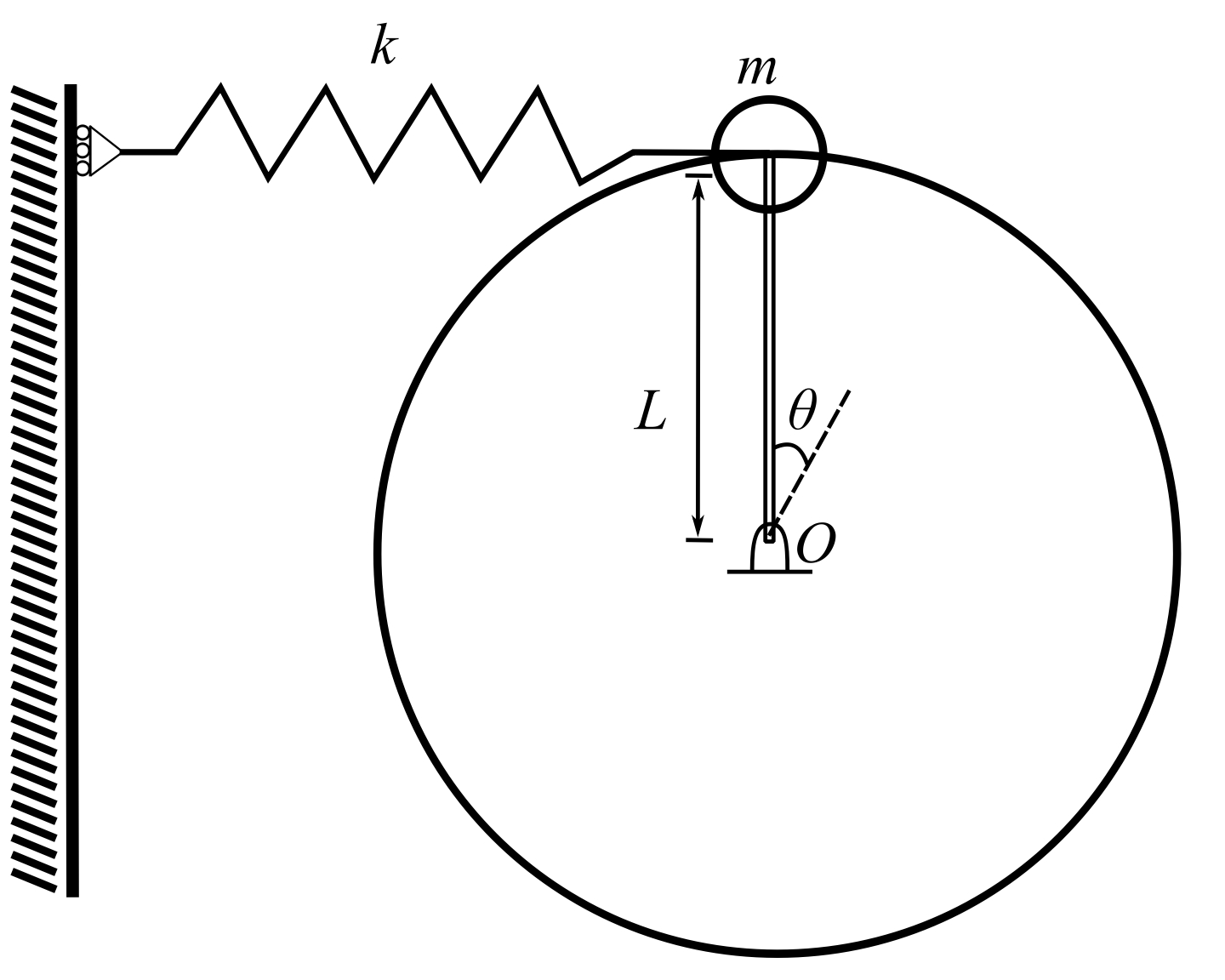
Solution

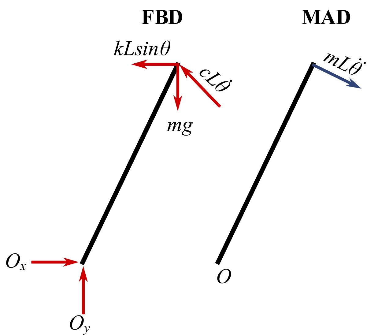
This image has an empty alt attribute; its file name is part1fig2_2.jpg

$\begin{split}+\circlearrowright \sum{M_0}& = mL^2\ddot{\theta} \\& = mgL\sin{\theta}-kL\sin{\theta}(L\cos{\theta}) - cL^2\ddot{\theta}\end{split}$

$mL^2 \ddot{\theta}+kL^2 \sin{\theta}\cos{\theta}- mgL\sin{\theta}+cL^2 \dot{\theta}=0$

$\ddot{\theta}+\frac{k}{m}\sin{\theta}\cos{\theta}-\frac{g}{L}\sin{\theta}+\frac{c}{m}\dot{\theta}=0 \quad (1)$

We must find static equilibrium configurations and determine equation of motion for small perturbations about these static configurations.

Set $\ddot{\theta} = \dot{\theta} = 0$ , and let $\theta = \theta_0$ . Therefore:

$\frac{k}{m} \sin{\theta_0} \cos{\theta_0} = \frac{g}{L} \sin{\theta_0}$

$\sin{\theta_0}\Big[\frac{k}{m}\cos{\theta_0}-\frac{g}{L}\Big] = 0$

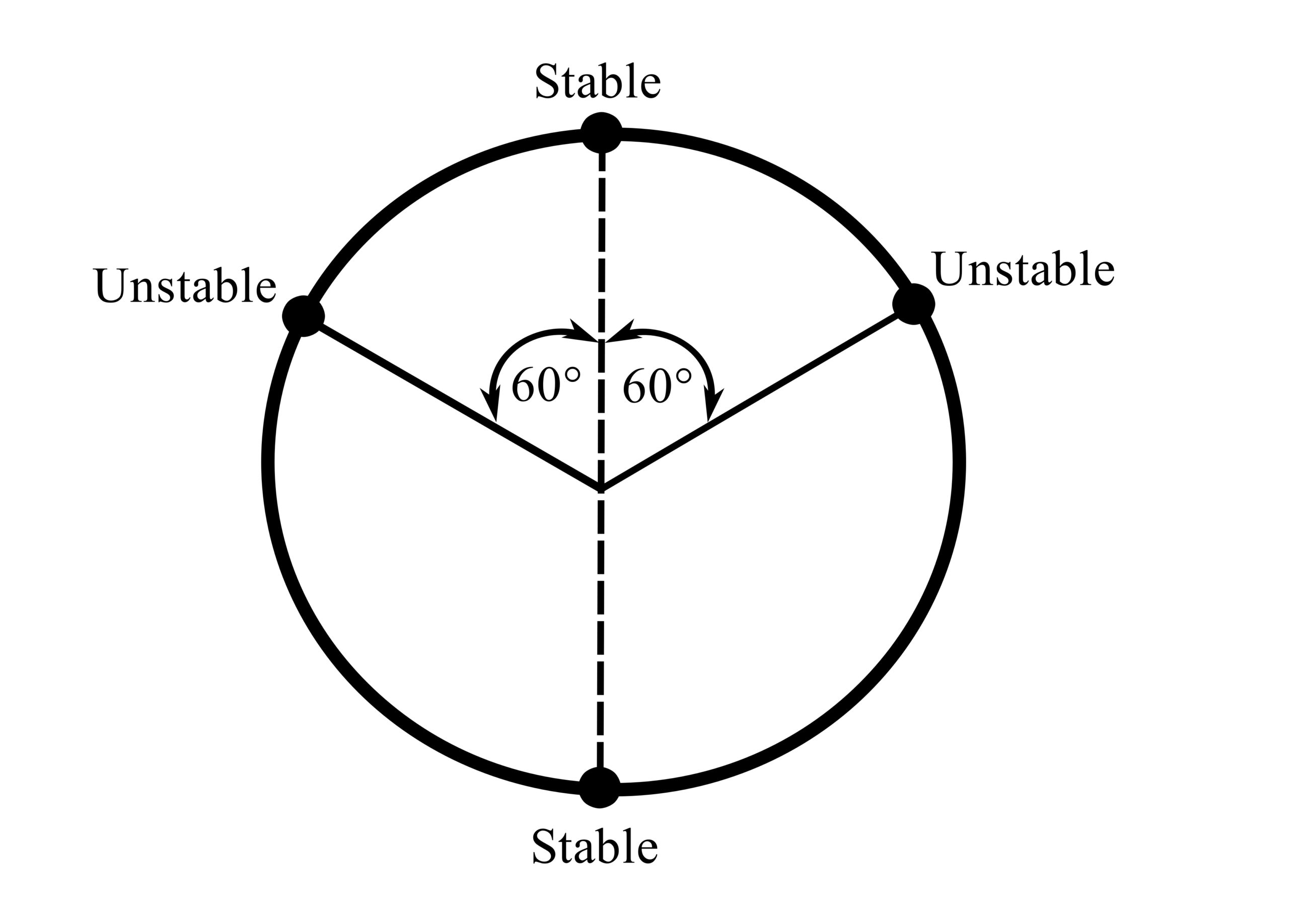
Therefore. the static configurations are given by:

$\theta_0 = 0, \pi \quad \sin{\theta_0}=0 \quad \cos{\theta_0} = \frac{mg}{kL}$

Assuming $\frac{mg}{kL}<1$ , there are 3 positions.

To find the motion, linearize (1) about $\theta_0$ . Set $\theta = \theta_0 + \hat{\theta}$ , where $\hat{\theta}$ is a small angle.

$\sin \theta = \sin(\theta_o + \hat{\theta}) \approx \sin \theta_o +\hat{\theta} \cos \theta_o$

$\cos \theta \approx \cos \theta_o - \hat{\theta}\sin\theta_o$

Put the above into the original equation of motion to get:

$\ddot{\hat{\theta}} + \frac {k}{m}(\sin \theta_o + \hat{\theta} \cos \theta_o)(\cos \theta_o - \hat{\theta}\sin \theta_o) - \frac{g}{L}(\sin \theta_o + \hat{\theta}\cos \theta_o) = 0$

Note that $\dot{\theta_o} = \ddot{\theta_o} = 0$ .

$\ddot{\hat{\theta}} + \frac {k}{m}(\sin \theta_o \cos \theta_o + \hat{\theta} \cos^2\theta_o - \hat{\theta}\sin^2\theta_o-\hat{\theta}^2\sin\theta_o \cos\theta_o) - \frac{g}{L}(\sin \theta_o + \hat{\theta}\cos \theta_o) + \frac{c}{m}\dot{\hat{\theta}} = 0$

Using the fact that the $\hat{\theta}^2$ term is small compared to 1, it becomes:

$\ddot{\hat{\theta}} + \Big(\frac{k}{m}\cos\theta_o - \frac{g}{L}\Big)\sin\theta_o + \hat{\theta}(\cos^2\theta_o-\sin^2\theta_o)\frac{k}{m} - \frac{g}{L}\hat{\theta}\cos\theta + \frac{c}{m}\dot{\hat{\theta}} = 0$

$\ddot{\hat{\theta}} + \hat{\theta}\Big(\frac{k}{m}\cos2\theta_o - \frac{g}{L}\cos\theta_o\Big) + \frac{c}{m}\dot{\hat{\theta}} + \Big(\frac{k}{m}\cos\theta_o - \frac{g}{L}\Big)\sin\theta_o = 0$

The above equation looks like the standard form except for a constant term that is zero for all conditions.

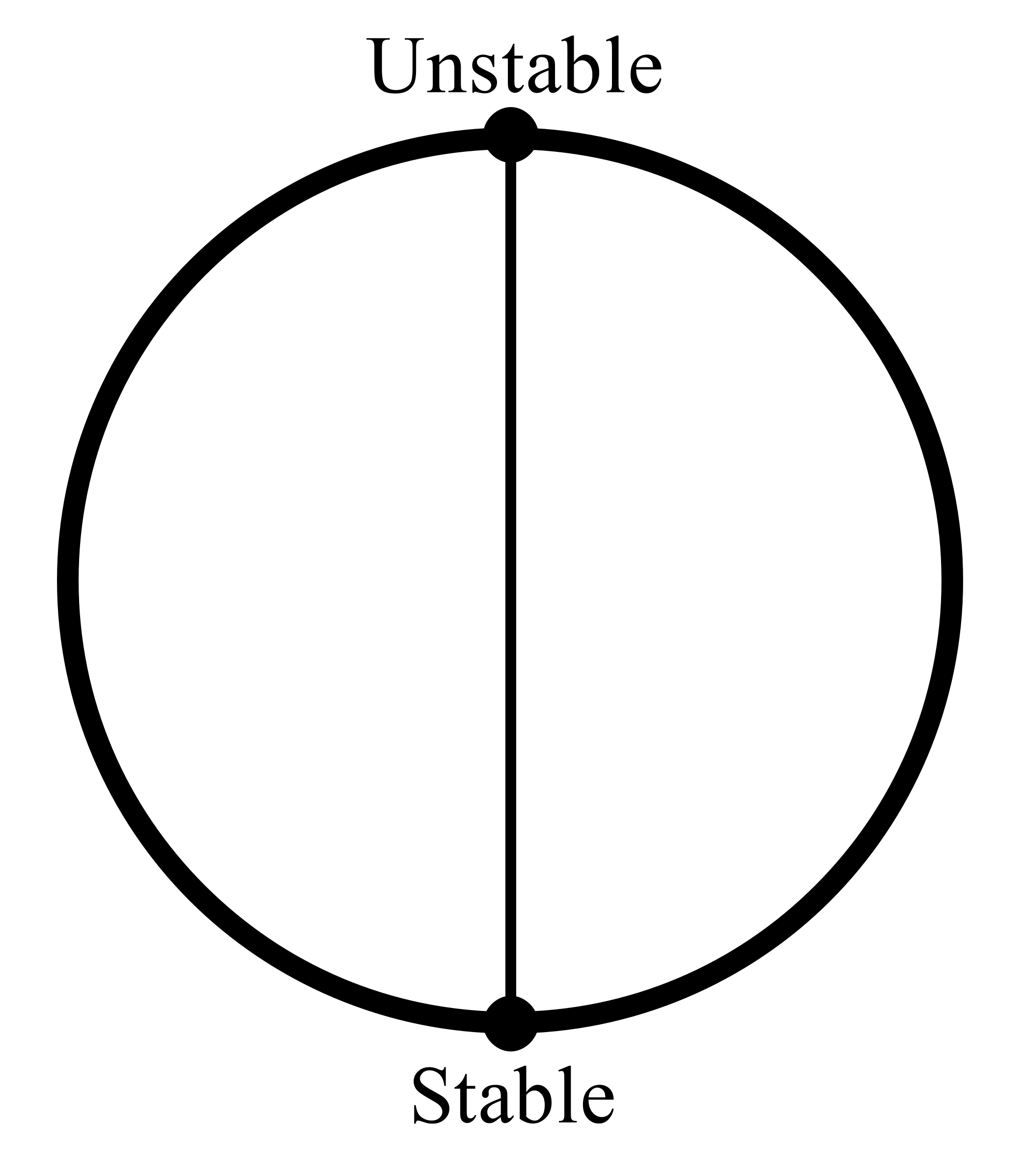
Now consider all three positions:

1. $\theta_o = 0$ .

$\ddot{\hat{\theta}} + \Big(\frac{k}{m} - \frac{g}{L}\Big)\hat{\theta} + \frac{c}{m}\dot{\hat{\theta}} = 0$

Therefore, this is stable if $\frac{k}{m} > \frac{g}{L}$ as $\frac{c}{m} > 0$ , but unstable if $\frac{k}{m} < \frac{g}{L}$ .

2. $\theta_o = \pi$ .

$\ddot{\hat{\theta}} + \Big(\frac{k}{m} + \frac{g}{L}\Big)\hat{\theta} + \frac{c}{m} = 0$

Therefore, this is always stable.

3. $\cos\theta_o = \frac{mg}{kL}$ .

$\ddot{\hat{\theta}} + \frac{k}{m}\Big(2\cos^2\theta_o - 1 - \frac{gm}{kL}\cos\theta_o\Big)\hat{\theta} + \frac{c}{m}\dot{\hat{\theta}} = 0$

$\ddot{\hat{\theta}} + \frac{k}{m}(\cos^2\theta_o - 1)\hat{\theta} + \frac{c}{m}\dot{\hat{\theta}} = 0$

Therefore, this is always unstable, regardless of damping.

Example

1. $\frac{mg}{kL} = \frac{1}{2}$ , $\theta_o = \pm 60^{\circ}$ , $\frac{k}{m} = \frac{2g}{L}$ . Therefore:

$\frac{k}{m} > \frac{g}{L}$

This image has an empty alt attribute; its file name is part1fig3-2-scaled.jpg

2. $\frac{mg}{kL} = 2$ , $\frac{k}{m} = \frac{1}{2}\frac{g}{L}$ . Therefore:

$\frac{k}{m} < \frac{g}{L}$

This image has an empty alt attribute; its file name is part1fig3_2-2.jpg

Open Educational Resources

Review of single and multi-degree of freedom (mdof) systems: Introduction and Review

Example

Solution

Example

Leave a Reply Cancel reply