
Review of single and multi-degree of freedom (mdof) systems: Vibration and Applications of MDOF Systems
For more than a SDOF system the analysis requires a more generalized approach. However, overall it doesn’t matter if there are 2 or 22 DOFs. Consider first a special 2 DOF free vibration system:
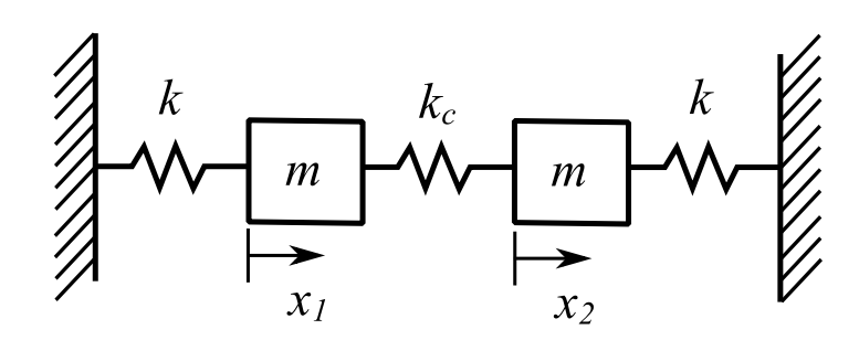
![\[ \begin{bmatrix} m & 0 \\ 0 & m \end{bmatrix} \begin{Bmatrix} \ddot{x_1} \\ \ddot{x_2} \end{Bmatrix} + \begin{bmatrix} k + k_c & -k_c \\ -k_c & k + k_c \end{bmatrix} \begin{Bmatrix} x_1 \\ x_2 \end{Bmatrix} = \begin{Bmatrix} 0 \\ 0 \end{Bmatrix}\]](https://engcourses-uofa.ca/wp-content/ql-cache/quicklatex.com-929db364452cb2df16884d49c78ccc53_l3.png "Rendered by QuickLaTeX.com")
The simplest approach is to look for Simultaneous Simple Harmonic Motion (SSHM). That is:
![\[ \begin{Bmatrix} x_1 \\ x_2 \end{Bmatrix} = \begin{Bmatrix} X_1 \\ X_2 \end{Bmatrix} \sin(pt + \phi) \]](https://engcourses-uofa.ca/wp-content/ql-cache/quicklatex.com-87714ef38610e9b08c2a1b890c400878_l3.png "Rendered by QuickLaTeX.com")
Which is a solution (not the general one) if:
![\[ \begin{bmatrix} k+k_c - mp^2 & -k_c \\ -k_c & k+k_c-mp^2 \end{bmatrix} \begin{Bmatrix} X_1 \\ X_2 \end{Bmatrix} = \begin{Bmatrix} 0 \\ 0 \end{Bmatrix} \]](https://engcourses-uofa.ca/wp-content/ql-cache/quicklatex.com-85efe386c8a77feb954beba2546242b7_l3.png "Rendered by QuickLaTeX.com")
This can be true if and only if (iff), ![\text{det}[] = 0](https://engcourses-uofa.ca/wp-content/ql-cache/quicklatex.com-f05067a0fe6327400f9e40e4d343ab21_l3.png "Rendered by QuickLaTeX.com") . Therefore:
. Therefore:
![\[ p^4-p^2\Big[\frac{(k+k_c)}{m} + \frac{(k+k_c)}{m}\Big] + \frac{k^2+2k_c k}{m^2} = 0 \]](https://engcourses-uofa.ca/wp-content/ql-cache/quicklatex.com-39c028c47e5dca4954bfefdd99c0034a_l3.png "Rendered by QuickLaTeX.com")
There are two soloutions for  .
.
![\[ \begin{split} p_{1,2}^2 &= \frac{k+k_c}{m} \pm \sqrt{\frac{k^2+2kk_c + k_c^2 - (k^2 + 2kk_c)}{m^2}} \\&= \frac{k+k_c}{m} \pm \frac{k_c}{m} \\&= \frac{k}{m}, \ \frac{k+2k_c}{m} \end{split}\]](https://engcourses-uofa.ca/wp-content/ql-cache/quicklatex.com-634f829480b55d4f948d3d5022accc12_l3.png "Rendered by QuickLaTeX.com")
Therefore:
![\[p_1 = \sqrt{\frac{k}{m}}, \ p_2 = \sqrt{\frac{k+2k_c}{m}} \]](https://engcourses-uofa.ca/wp-content/ql-cache/quicklatex.com-6cb208f9268c14b23ba47317fa8bb12b_l3.png "Rendered by QuickLaTeX.com")
As a result, there are 2 frequencies at which our assumption is true. NOTE: It turns out that the general solution can be determined from these  ,
,  , and the ratio of the amplitudes between the two masses during each of the two SSHMs. Therefore:
![\[ (k + k_c - mp^2)X_1 -k_cX_2 = 0 \]](https://engcourses-uofa.ca/wp-content/ql-cache/quicklatex.com-760bbef2456770ed44b5eba30d798381_l3.png "Rendered by QuickLaTeX.com")
Or:
![\[ -k_cX_1 + (k + k_c - mp^2)X_2 = 0 \]](https://engcourses-uofa.ca/wp-content/ql-cache/quicklatex.com-8f9f2d91c213bc0f251ce36039461d8d_l3.png "Rendered by QuickLaTeX.com")
Therefore, for either  or
or  :
:
![\[ \begin{split} \frac{X_2}{X_1} &= \frac{k +k_c -mp^2}{k_c} \\&= \frac{k_c}{k+k_c-mp^2} \end{split} \]](https://engcourses-uofa.ca/wp-content/ql-cache/quicklatex.com-328e44d8a089158705e8ee12c0d62183_l3.png "Rendered by QuickLaTeX.com")
If we put into either we get:
![\[ \Big(\frac{X_2}{X_1}\Big)_1 = \frac{1}{1} \equiv X_1 \]](https://engcourses-uofa.ca/wp-content/ql-cache/quicklatex.com-5ab1a785cddf70ee80d7ea3aaef229ae_l3.png "Rendered by QuickLaTeX.com")
And if we put into either we get:
![\[ \Big(\frac{X_2}{X_1}\Big)_2 = \frac{-1}{1} \equiv X_2 \]](https://engcourses-uofa.ca/wp-content/ql-cache/quicklatex.com-81f85416eebf8603da3e82d6cf8e5c1c_l3.png "Rendered by QuickLaTeX.com")
Thus, we define the mode shapes corresponding to each ratio:
![\[ \{u\}_1 = \begin{Bmatrix} 1 \\ X_1 \end{Bmatrix} \]](https://engcourses-uofa.ca/wp-content/ql-cache/quicklatex.com-b8e0e2588bf3323df531f921f77a0d6a_l3.png "Rendered by QuickLaTeX.com")
![\[ \{u\}_2 = \begin{Bmatrix} 1 \\ X_2 \end{Bmatrix} \]](https://engcourses-uofa.ca/wp-content/ql-cache/quicklatex.com-ab91a0c2f62bc93efb83882915e04eaf_l3.png "Rendered by QuickLaTeX.com")
Therefore, we have a mode shape corresponding to each of the natural frequencies.  and
and  are “normalized” vectors where the first component is set arbitrarily to unity. The general solution to the free vibration problem is then:
![\[ \begin{Bmatrix} x_1 \\ x_2 \end{Bmatrix} = c_1 \{u\}_1 \sin(p_1t +\phi_1) + c_2\{u\}_2 \sin(p_2t+\phi_2) \]](https://engcourses-uofa.ca/wp-content/ql-cache/quicklatex.com-c40f423b00b757ff86df1699aecf4d59_l3.png "Rendered by QuickLaTeX.com")
There are 4 constants  ,
,  ,
,  ,
,  for the 4 initial conditions for
  ,
,  ,
,  ,
,  . If the initial conditions are selected then the solution will include both modes in general but only one mode for certain cases. (For example, when
  ,
,  ,
,  , and
, and  ,
,  mode 1).
Consider the following initial conditions:
![\[x_1(0) = 1,\ x_2(0) = 0,\ \dot{x}_1(0) = 0,\ \dot{x}_2(0) = 0\]](https://engcourses-uofa.ca/wp-content/ql-cache/quicklatex.com-8bc8c149d6df5f2cc9303e824048e5e8_l3.png "Rendered by QuickLaTeX.com")
![\[x_1(t) = c_1\sin(p_1t+\phi_1) + c_2\sin(p_2t+\phi_2) \]](https://engcourses-uofa.ca/wp-content/ql-cache/quicklatex.com-fce5b47300a026ca9d3637c6c66a0f62_l3.png "Rendered by QuickLaTeX.com")
![\[x_2(t) = c_1\sin(p_1t+\phi_1) - c_2\sin(p_2t+\phi_2) \]](https://engcourses-uofa.ca/wp-content/ql-cache/quicklatex.com-ac32f1604a8ff4948a89b502e59b3cf9_l3.png "Rendered by QuickLaTeX.com")
At  :
:
![\[1 = c_1\sin\phi_1 + c_2\sin\phi_2 \quad (1) \]](https://engcourses-uofa.ca/wp-content/ql-cache/quicklatex.com-66b69e8b972bab93026f9d5d3c4831b6_l3.png "Rendered by QuickLaTeX.com")
![\[0 = c_1\sin\phi_1 - c_2\sin\phi_2 \quad (2) \]](https://engcourses-uofa.ca/wp-content/ql-cache/quicklatex.com-b0d6c50c5aa1ff13986b654d16995d8a_l3.png "Rendered by QuickLaTeX.com")
![\[0 = p_1\cos\phi_1 + p_2\cos\phi_2 \quad (3) \]](https://engcourses-uofa.ca/wp-content/ql-cache/quicklatex.com-a8b99e32f6f04e52caa9cfb3fa53dc12_l3.png "Rendered by QuickLaTeX.com")
![\[0 = p_1\cos\phi_1 - p_2\cos\phi_2 \quad (4) \]](https://engcourses-uofa.ca/wp-content/ql-cache/quicklatex.com-5aae6896650bc7c010d846d901c352f5_l3.png "Rendered by QuickLaTeX.com")
Therefore:
![\[ \cos\phi_1 = 0 \quad ((3) + (4)) \]](https://engcourses-uofa.ca/wp-content/ql-cache/quicklatex.com-754540f5dcec437cee0432c4fa3a730f_l3.png "Rendered by QuickLaTeX.com")
![\[ \cos\phi_2 = 0 \quad ((3) - (4)) \]](https://engcourses-uofa.ca/wp-content/ql-cache/quicklatex.com-a22c700839a8bb8740db3b29a3957e61_l3.png "Rendered by QuickLaTeX.com")
Therefore:
![\[ \phi_1 = \frac{\pi}{2},\ \phi_2 = \frac{\pi}{2}\]](https://engcourses-uofa.ca/wp-content/ql-cache/quicklatex.com-3386dfdc5a08b72e1aa2abd5ad06cb01_l3.png "Rendered by QuickLaTeX.com")
From (1) and (2) (+):
![\[2c_1\sin\phi_1 = 1\]](https://engcourses-uofa.ca/wp-content/ql-cache/quicklatex.com-5acc82bcfb72f9ba623c220bf0da3985_l3.png "Rendered by QuickLaTeX.com")
![\[c_1 = \frac{1}{2}\]](https://engcourses-uofa.ca/wp-content/ql-cache/quicklatex.com-e044f60ad40ea00765bc6a7b5d2ba65c_l3.png "Rendered by QuickLaTeX.com")
From (1) and (2) (-):
![\[c_2 = \frac{1}{2}\]](https://engcourses-uofa.ca/wp-content/ql-cache/quicklatex.com-24da893f4515bee85cdb8441abb44fc5_l3.png "Rendered by QuickLaTeX.com")
Therefore:
![\[\begin{split} x_1 &= \frac{1}{2}\sin\Big(p_1t + \frac{\pi}{2}\Big) + \frac{1}{2}\sin\Big(p_2t + \frac{\pi}{2}\Big) \\&= \frac{1}{2}\cos p_1t + \frac{1}{2}\cos p_2t \end{split} \]](https://engcourses-uofa.ca/wp-content/ql-cache/quicklatex.com-7c2c85accd5775261cf0d4d13e2843c4_l3.png "Rendered by QuickLaTeX.com")
![\[x_2 = \frac{1}{2}\cos p_1t - \frac{1}{2}\cos p_2t \]](https://engcourses-uofa.ca/wp-content/ql-cache/quicklatex.com-cd48ce70f4fef97abdb0555247121c69_l3.png "Rendered by QuickLaTeX.com")
Using identities:
![\[x_1 = \Big[\cos(p_2-p_1)\frac{t}{2} \bullet \cos(p_1+p_2)\frac{t}{2}\Big] \]](https://engcourses-uofa.ca/wp-content/ql-cache/quicklatex.com-188bc7da0142922eeb1a3d106c394485_l3.png "Rendered by QuickLaTeX.com")
![\[x_2 = \Big[\sin(p_2-p_1)\frac{t}{2} \bullet \sin(p_2+p_1)\frac{t}{2}\Big] \]](https://engcourses-uofa.ca/wp-content/ql-cache/quicklatex.com-2d15eb10222c5dd2e17e099fb7429a79_l3.png "Rendered by QuickLaTeX.com")
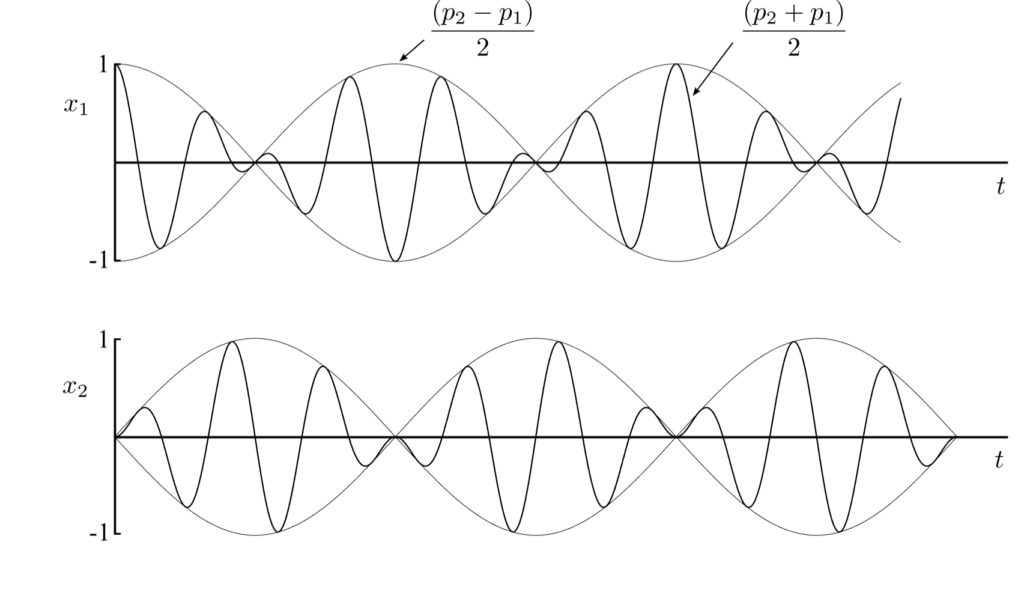
These may be interpreted as a higher frequency oscillation at the average of the two natural frequencies with a variable amplitude, given by a lower frequency given by  the difference in natural frequencies.
If and are close to each relative to their magnitude then  , the motion becomes:
if sinx(x)=-cos(x+pi/2)
Could it be x1 and x2 negative?
Sorry
sin(x)=-cos(x+pi/2)
Ok.I’m wrong
sin(x+pi/2)=cos(x)
Could it be x1 and x2 were positive
Thanks a lot for the classes.
Best regards