
Advanced Dynamics and Vibrations: Lagrange’s equations applied to dynamic systems
Analytical Mechanics – Lagrange’s Equations
Up to the present we have formulated problems using newton’s laws in which the main disadvantage of this approach is that we must consider individual rigid body components and as a result, we must deal with interaction forces that we really have no interest in. These forces come from constraints which one part of the system puts on another.
An alternate approach referred to as analytical mechanics, considers the system as a whole and formulates the equations of motion starting from scalar quantities – the kinetic and potential energies and an expression of the virtual work associated with non-conservative forces. It relies heavily on the concept of virtual displacements.
Any set of numbers that serve to specify the configuration of the system are examples of generalized coordinates. To these we can add constraints. The number of DOF is then the number of generalized coordinates minus the number of independent equations of constraint.
e.g a point moving on the surface of a sphere of radius R with center  must obey:
![\[(x-x_{0})^{2} + (y-y_{0})^{2} + (z- z _{0})^{2} = R^{2}\]](https://engcourses-uofa.ca/wp-content/ql-cache/quicklatex.com-1cf9b78ef46e8104eca01a0625bbffeb_l3.png "Rendered by QuickLaTeX.com")
There are 3 coordinates and 1 equation of constraint. Therefore it has 2 DOF. If we used two angles, say  &
&  then we would not need the constraint.
These constraints are classified as:
 If the constraint can be written in finite form (as above) they are called holonomic if not (then in differential form) then they are non-holonomic.
 If they are equalities then they are bilateral and unilateral if inequalities
 If there is no explicit dependence on time then they are scleronomic and if there is explicit time dependence they are rheonomic.
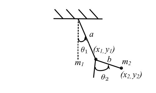
![\[x_{1}^{2} + y_{1}^{2} = a^{2}\]](https://engcourses-uofa.ca/wp-content/ql-cache/quicklatex.com-41f133ab0a2053559cede985176780ff_l3.png "Rendered by QuickLaTeX.com")
![\[(x_{2} - x_{1})^{2} + (y_{2} - y_{1})^{2} = b^{2}\]](https://engcourses-uofa.ca/wp-content/ql-cache/quicklatex.com-8ca5e759ced3b38eb1fb298114f9eed0_l3.png "Rendered by QuickLaTeX.com")
Therefore, 2 DOF holonomic, scleronomic bilateral system.
 (unilateral)
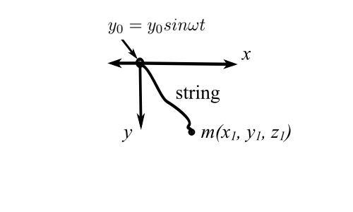
however if we allow the point of attachment to move (in the x-y plane)
 (rheonomic)
Vertical displacement & Virtual Work
The work done during the motion is
![\[\overline{d W} = \underline{F} \cdot d \underline{r}\]](https://engcourses-uofa.ca/wp-content/ql-cache/quicklatex.com-2d6590468a2f3bd3da096f281a3a6f7a_l3.png "Rendered by QuickLaTeX.com")
where  &
&  are vectors and
  is a scalar. For a particle
  where may be the sum of several forces. Therefore,
![\[\begin{split} \overline{dW} &= m \ddot{\underline{r}} \cdot dr \\&= m \frac{d \dot{\underline{r}}}{dt} \cdot ( \frac{d \underline{r}}{dt}dt) \\&= m \frac{d \dot{r}}{dt} \cdot (\dot{r} dt) \\&= m \dot{\underline{r}} \cdot d \dot{r} \\&= d(\frac{1}{2} m \dot{\underline{r}} \cdot \dot{\underline{r}})\end{split}\]](https://engcourses-uofa.ca/wp-content/ql-cache/quicklatex.com-176932b338ffdc4588f574e4016718df_l3.png "Rendered by QuickLaTeX.com")
where this is a true differential of the kinetic energy.
![\[T = \frac{1}{2} m \dot{\underline{r}} \cdot \dot{\underline{r}}\]](https://engcourses-uofa.ca/wp-content/ql-cache/quicklatex.com-2abf636831f876f17312fa9a0042bda9_l3.png "Rendered by QuickLaTeX.com")
If the particle moves from positive  to
to  then
then
![\[\int_{\underline{r}_{1}}^{\underline{r}_{2}} \underline{F} \cdot d \underline{r} = \frac{1}{2} m [\underline{\dot{r}}_{2} \cdot \underline{\dot{r}}_{2}] - \frac{1}{2} m [\underline{\dot{r}}_{1} \cdot \underline{\dot{r}}_{1}]\]](https://engcourses-uofa.ca/wp-content/ql-cache/quicklatex.com-a57aea13ce48abc3d69b57e000c74076_l3.png "Rendered by QuickLaTeX.com")
if depends only on  ,
, 
![\[dW = F \cdot d \underline{r} \equiv -dV(\underline{r})\]](https://engcourses-uofa.ca/wp-content/ql-cache/quicklatex.com-5ccaa0f5b274ab106842577208a75b37_l3.png "Rendered by QuickLaTeX.com")
where  is a scalar function that depends only on the position and not on
  or time.
  is term the potential energy.
![\[d(T+V) = 0\]](https://engcourses-uofa.ca/wp-content/ql-cache/quicklatex.com-c726b0773cf601834e71f03ed3e3deca_l3.png "Rendered by QuickLaTeX.com")
The total energy is constant.
When we have a conservative system we can use Rayleigh’s to estimate the natural frequencies.
Consider a simple problem and use visual work to solve.
Two bars of length  . What is the equilibrium position
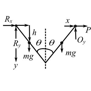
Therefore,
![\[P \delta x + 2mg \delta h = 0\]](https://engcourses-uofa.ca/wp-content/ql-cache/quicklatex.com-8f5a9cfa82a5bcd2385e7817866b65dc_l3.png "Rendered by QuickLaTeX.com")
![\[x = 2 \ell \sin \theta\]](https://engcourses-uofa.ca/wp-content/ql-cache/quicklatex.com-405b69437e307807c1d98853a520cb6b_l3.png "Rendered by QuickLaTeX.com")
![\[h = \frac{\ell}{2} \cos \theta\]](https://engcourses-uofa.ca/wp-content/ql-cache/quicklatex.com-5e2181fd63aa2e386f456a94d71817c2_l3.png "Rendered by QuickLaTeX.com")
![\[\delta x = 2\ell \cos \theta \delta \theta\]](https://engcourses-uofa.ca/wp-content/ql-cache/quicklatex.com-8a12c62b66eb1b003caff668a8911b88_l3.png "Rendered by QuickLaTeX.com")
![\[\delta h = \frac{- \ell}{2} \sin \theta \delta \theta\]](https://engcourses-uofa.ca/wp-content/ql-cache/quicklatex.com-91233cd570f82206eed1247f528990db_l3.png "Rendered by QuickLaTeX.com")
![\[P(2 \ell \cos \theta \delta \theta) = 2mg(\frac{\ell}{2} \sin \theta \delta \theta)\]](https://engcourses-uofa.ca/wp-content/ql-cache/quicklatex.com-086d02206eb1a200261f31b6cf88c07e_l3.png "Rendered by QuickLaTeX.com")
![\[\frac{P}{mg} = \tan \theta\]](https://engcourses-uofa.ca/wp-content/ql-cache/quicklatex.com-f37f143a1ef6d3d5b5f4b899e1380918_l3.png "Rendered by QuickLaTeX.com")
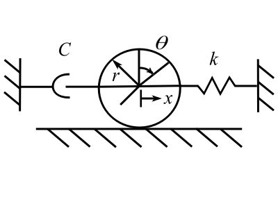
Consider a rigid beam (uniform) of mass  loaded by a uniform time dependent load
  and supported by a spring & dashpot as shown
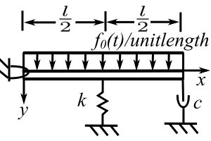
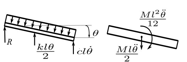
Using  determine the equation of motion.
 Virtual work of forces applied
  Virtual work of inertia forces
![\[\frac{-kl \theta}{2}\Big( \frac{\ell \delta \theta}{2} \Big) - cl \dot{\theta}(l \delta \theta) + \int_{0}^{l} f_{o}(t)dx (x \delta \theta) = \frac{Ml^{2}}{12} \ddot{\theta} \delta \theta + M \frac{l \ddot{\theta}}{2} \Big( \frac{l}{2} \delta \theta \Big) \]](https://engcourses-uofa.ca/wp-content/ql-cache/quicklatex.com-50deb3dec231b2b1f70f05a88b80e386_l3.png "Rendered by QuickLaTeX.com")
Therefore,
![\[M \ell^{2}\Big[ \frac{1}{12} + \frac{1}{4}\Big] \ddot{\theta} \delta \theta + \frac{k \ell^{2}}{4} \theta \delta \theta + c \ell^{2} \dot{\theta} \delta \theta = f_{o}(t) \frac{ \ell^{2}}{2} \delta \theta\]](https://engcourses-uofa.ca/wp-content/ql-cache/quicklatex.com-fa39a094bd538e9e1fb3dbd55c857599_l3.png "Rendered by QuickLaTeX.com")
![\[ \frac{M}{3} \ddot{\theta} + c \dot{\theta} + \frac{k}{4} \theta = \frac{f(t)}{2}\]](https://engcourses-uofa.ca/wp-content/ql-cache/quicklatex.com-ffed38ea38e1c5869d811d54e0994102_l3.png "Rendered by QuickLaTeX.com")
We can use virtual work to calculate the energy in a multi-degree of freedom system.
For a displacement of  only
only
![\[F_{1} = k_{11} \delta _{1} \hspace{1cm} F_{2} = k_{21} \delta _{1} \hspace{1cm} F_{3} = k_{31} \delta _{1}\]](https://engcourses-uofa.ca/wp-content/ql-cache/quicklatex.com-dbfd3c2c2aacf8984075cb0ad1efac19_l3.png "Rendered by QuickLaTeX.com")
and similarly for  ,
,  alone
alone
![\[F_{1} = k_{12} \delta _{2} \hspace{1cm} F_{2} = k_{22} \delta _{2} \hspace{1cm} F_{3} = k_{32} \delta _{2}\]](https://engcourses-uofa.ca/wp-content/ql-cache/quicklatex.com-782c4ce90e05584e73731ca9d4311fbe_l3.png "Rendered by QuickLaTeX.com")
![\[F_{1} = k_{13} \delta _{3} \hspace{1cm} F_{2} = k_{23} \delta _{3} \hspace{1cm} F_{3} = k_{33} \delta _{3}\]](https://engcourses-uofa.ca/wp-content/ql-cache/quicklatex.com-7d5534bb0c0d331637000cb289a773a4_l3.png "Rendered by QuickLaTeX.com")
So for the combination (assuming superposition)
![\[F_{i} = \sum _{j=1}^{n} k_{ij} \delta _{j}\]](https://engcourses-uofa.ca/wp-content/ql-cache/quicklatex.com-cfe667d154f53688ecd53aa38a51d3c8_l3.png "Rendered by QuickLaTeX.com")
and
![\[\delta _{i} = \sum _{j=1}^{n} a_{ij} F _{j}\]](https://engcourses-uofa.ca/wp-content/ql-cache/quicklatex.com-5c04ac541feb0dad8b4c5c8ab8541986_l3.png "Rendered by QuickLaTeX.com")
The work done by force  in
in  is energy stored due to that force:
![\[V_{i} = \frac{1}{2} F_{i} \delta _{i}\]](https://engcourses-uofa.ca/wp-content/ql-cache/quicklatex.com-86361ace92dd259db969c45a27819e45_l3.png "Rendered by QuickLaTeX.com")
If there are n forces and the displacements are (i = 1,2, … n) then the total energy is:
![\[\begin{split} V &= \sum _{i=1}^{n} V_{i} \\&= \frac{1}{2} \sum _{i=1}^{n} F_{i} \delta _{i} \\&= \frac{1}{2} \sum _{i=1}^{n} \Bigg( \sum _{j=1}^{n} k_{ij} \delta _{j} \Bigg) \delta _{i} \end{split}\]](https://engcourses-uofa.ca/wp-content/ql-cache/quicklatex.com-7403cff018eb6d4ae73bb5b75c7e6cbf_l3.png "Rendered by QuickLaTeX.com")
![\[\begin{split} V &= \frac{1}{2} \{\delta \}^{T} [k] \{ \delta\} \\&= \frac{1}{2} \{F \}^{T} [a] \{ F\} \end{split}\]](https://engcourses-uofa.ca/wp-content/ql-cache/quicklatex.com-fa3601324d0e34221a81937eb8ab3a8f_l3.png "Rendered by QuickLaTeX.com")
We can also show that the kinetic energy is
![\[T = \frac{1}{2} \{\dot{\delta}\}^{T} [m] \{\dot{\delta}\}\]](https://engcourses-uofa.ca/wp-content/ql-cache/quicklatex.com-6467dfa97597dd7a57266aa2c8617c36_l3.png "Rendered by QuickLaTeX.com")
 & are examples of so-called quadratic forms. Quadratic forms are said to be positive definite if they are never negative and only zero when the variables are zero (
 )
)
They are said to be positively semi-definite if they are never negative but can be zero for non-negative variables.
This is useful to know because if we have a stiffness matrix that is positive semi-definite it means there is a rigid body mode with zero natural frequency  [m] is positive definite
 ![]](https://engcourses-uofa.ca/wp-content/ql-cache/quicklatex.com-9078c1820ad5ee29ecec7cc9c1e062dc_l3.png "Rendered by QuickLaTeX.com")
For example a submarine:
has 2 rigid body modes
Principle of Virtual Work
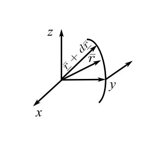
We will consider a system of  particles moving in a 3D space and define the virtual displacements as
  for particle 1
  for particle 2 etc.
These are not true displacements but small variations in the so-called generalized coordinates. These are imagined displacements (slight variations) which are at the same time and which satisfy the constraints given by
![\[g_{j} (x_{1}, y_{1}, z _{1}, x_{2}, y_{2}, z _{2} ..... t) = c \hspace{1cm} j = 1\quad \text{to} \quad m\]](https://engcourses-uofa.ca/wp-content/ql-cache/quicklatex.com-4df8f8db0dded617ec52644bc8a96f2a_l3.png "Rendered by QuickLaTeX.com")
Then for virtual changes in these coordinates:
![\[g_{j} (x_{1} + \delta x_{1} , y_{1} + \delta y_{1}, z _{1} + \delta z _{1} ..... t) = c \]](https://engcourses-uofa.ca/wp-content/ql-cache/quicklatex.com-75e2dd89603f04933b409ac1ec1dbc9e_l3.png "Rendered by QuickLaTeX.com")
Expanding this in a Taylor series gives:
![\[g_{j}(x_{1}, y_{1}, \zeta _{1},..... t) + \sum _{i=1} ^{N} \frac{\partial g_{i}}{\partial x_{i}} \delta x_{i} + \frac{\partial g_{j}}{\partial y_{i}} \delta y_{i} + \frac{\partial g_{j}}{\partial z_{i}} \delta z_{i} = C\]](https://engcourses-uofa.ca/wp-content/ql-cache/quicklatex.com-1b1c869e245b4e39f54d89e363f9a01d_l3.png "Rendered by QuickLaTeX.com")
Therefore,
![\[\sum _{i=1} ^{N} \frac{\partial g_{j}}{\partial x_{i}} \delta x_{i} + \frac{\partial g_{j}}{\partial y_{j}} \delta y_{j} + \frac{\partial g_{j}}{\partial z _{j}} \delta z _{j} = 0 \hspace{1cm} \forall _{j}\]](https://engcourses-uofa.ca/wp-content/ql-cache/quicklatex.com-b36152e7d28098a3cb271395addf867e_l3.png "Rendered by QuickLaTeX.com")
So that there are  arbitrary displacements
On each of these particles the forces acting are
![\[\underline{R}_{i} = \underline{F}_{i} + \underline{f}_{i} \hspace{1cm} i = 1,2, ... N\]](https://engcourses-uofa.ca/wp-content/ql-cache/quicklatex.com-586f7338420df47576db9a3139166f4c_l3.png "Rendered by QuickLaTeX.com")
Where the resultant force  is composed of the external forces
  and
and  the constraint forces.
When all the particles are in static equilibrium
![\[\underline{R}_{i} = 0 \hspace{1cm} \forall _{i}\]](https://engcourses-uofa.ca/wp-content/ql-cache/quicklatex.com-2602e19556a5daedf428dab4546c564d_l3.png "Rendered by QuickLaTeX.com")
and
![\[\underline{R}_{i} \cdot \delta \underline{r}_{i} = 0\]](https://engcourses-uofa.ca/wp-content/ql-cache/quicklatex.com-275a830deba2e6ff8f1c69a40e0c5bb8_l3.png "Rendered by QuickLaTeX.com")
where this represents the virtual work performed by the resultant force on the  particle.
![\[\delta \overline{W} = \sum _{i=1} ^{N} \underline{R}_{i} \cdot \delta \underline{r}_{i}\]](https://engcourses-uofa.ca/wp-content/ql-cache/quicklatex.com-d5e225eaef1920c1e10c28bce6cfb4d1_l3.png "Rendered by QuickLaTeX.com")
![\[\delta \overline{W} = \sum _{i=1} ^{N} \left(\underline{F}_{i} \cdot \delta \underline{r}_{i} + \underline{f}_{i} \cdot \delta \underline{r}_{i}\right) = 0\]](https://engcourses-uofa.ca/wp-content/ql-cache/quicklatex.com-1a960535ec3f257951aa29c8628573b0_l3.png "Rendered by QuickLaTeX.com")
If we rule out work by the constraint forces ( as the constraint force is perpendicular to the motion), (therefore cannot handle friction).
Consider two particles held by a rigid massless rod.
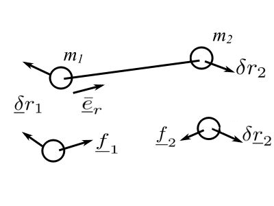
![\[|\underline{f} _{1}| = |\underline{f} _{2}|\]](https://engcourses-uofa.ca/wp-content/ql-cache/quicklatex.com-60d3c407babb21ee025136973ae06495_l3.png "Rendered by QuickLaTeX.com")
![\[\delta W = \underline{f}_{1} \cdot \underline{\delta} r_{1} + \underline{f}_{2} \cdot \underline{\delta} r_{2}\]](https://engcourses-uofa.ca/wp-content/ql-cache/quicklatex.com-e7e5198cb71eb56427eb84f7c47a8be4_l3.png "Rendered by QuickLaTeX.com")
But because the rod is rigid
![\[\delta \underline{r}_{1} \cdot \underline{e}_{r} = \delta \underline{r}_{2} \cdot \underline{e}_{r}\]](https://engcourses-uofa.ca/wp-content/ql-cache/quicklatex.com-64382e914b36a098d2a7523bebea93f0_l3.png "Rendered by QuickLaTeX.com")
![\[\delta W = f_{1} \underline{e}_{r} \cdot \delta \underline{r}_{1} - f_{2} \underline{e}_{r} \cdot \delta \underline{r}_{2}\]](https://engcourses-uofa.ca/wp-content/ql-cache/quicklatex.com-e804993142944b415c87cc6d8c6445ec_l3.png "Rendered by QuickLaTeX.com")
Therefore for the constraint forces
![\[\begin{split} \delta W &= (f_{1} - f_{2}) \underline{e}_{r} \cdot \delta r_{2} \\&= 0 \end{split}\]](https://engcourses-uofa.ca/wp-content/ql-cache/quicklatex.com-85aa0ca8b16d53e4eaa0ab8a94138b77_l3.png "Rendered by QuickLaTeX.com")
and the Principal of Virtual Work says
![\[\begin{split} \delta W &= \sum _{i=1} ^{N} \underline{F}_{i} \cdot \underline{\delta} r_{i}\\& = 0 \end{split}\]](https://engcourses-uofa.ca/wp-content/ql-cache/quicklatex.com-5635e1b62f701c49e2b7f3e3c04e3f82_l3.png "Rendered by QuickLaTeX.com")
that the work performed by the applied forces through infinitesimal virtual displacements compatible with the constraints is zero.
To make the virtual work equations more useful we write it in terms of the generalized coordinates 
![\[\begin{split} \delta W &= \sum _{i=1} ^{N} \underline{F}_{i} \cdot \delta r_{i} \\&= \sum _{i=1} ^{N} \underline{F}_i\cdot \sum _{j=1} ^{n} \frac{\partial \underline{r}_{i}}{\partial q_{j}} \delta q_{j} \\&= \sum _{j=1} ^{n} \Bigg( \sum _{i=1} ^{N} \underline{F}_i \cdot \frac{\partial \underline{r}_{i}}{\partial q_{j}} \Bigg) \delta q_{j} \end{split}\]](https://engcourses-uofa.ca/wp-content/ql-cache/quicklatex.com-f91c87c4f1e938db975ae7760a334ddc_l3.png "Rendered by QuickLaTeX.com")
We call
![\[Q_{j} =\sum _{i=1} ^{N} \underline{F}_{i} \cdot \frac{\partial \underline{r}_{i}}{\partial q_{j}}\]](https://engcourses-uofa.ca/wp-content/ql-cache/quicklatex.com-250537cd8e5db2b219e5cc2759c268d4_l3.png "Rendered by QuickLaTeX.com")
the generalized forces. These are not necessarily forces as they can be moments. It is only necessary that the quantity  has the units of work.
For the situation in which we have a conservative system the work can be expressed differently.
![\[\begin{split} \delta W &= \sum _{i=1} ^{N} \underline{F}_{i} \cdot \delta \underline{r}_{i} \\&= - \delta V \\&= - \sum _{i=1} ^{N} \Bigg( \frac{\partial V}{\partial x_{i}} \delta _{i} + \frac{\partial V}{\partial y_{i}} \delta y_{i} + \frac{\partial V}{\partial z _{i}} \delta z _{i} \Bigg) \\&= 0 \end{split}\]](https://engcourses-uofa.ca/wp-content/ql-cache/quicklatex.com-985d43ea2a948f1cbf55cbc835199cf7_l3.png "Rendered by QuickLaTeX.com")
as we can select the virtual displacement arbitrarily (i.e. only one non-zero at a time)
![\[\underline{F}_{x_{i}} = -\frac{\partial V}{\partial x_{i}} = 0, \hspace{0.5cm} \underline{F}_{y_{i}} = -\frac{\partial V}{\partial y_{i}} = 0, \hspace{0.5cm} \underline{F}_{z _{i}} = -\frac{\partial V}{\partial z _{i}} = 0\]](https://engcourses-uofa.ca/wp-content/ql-cache/quicklatex.com-265b8a1cae794c569b4fd903da03685c_l3.png "Rendered by QuickLaTeX.com")
This states that has a stationary value at the equilibrium position (can use this for stability consideration). To extend this to dynamical situations we use D’Alembert’s principle.
![\[\underline{F}_{i} +\underline{f}_{i} - m_{i} \underline{\ddot{r}}_{i} = 0\]](https://engcourses-uofa.ca/wp-content/ql-cache/quicklatex.com-74a00efcaf1edef87d99b1e07ab38aa3_l3.png "Rendered by QuickLaTeX.com")
Where the  are the inertia forces. The virtual work for a system of particles is:
![\[\sum _{i=1} ^{N} (\underline{F}_{i} +\underline{f}_{i} - m_{i} \underline{\ddot{r}}_{i}) \cdot \delta \underline{r}_{i} = 0\]](https://engcourses-uofa.ca/wp-content/ql-cache/quicklatex.com-a62a6a8161dfcac31759088b8868bc12_l3.png "Rendered by QuickLaTeX.com")
and since we showed the virtual work of the interned forces is zero.
![\[\sum _{i=1} ^{N} (\underline{F}_{i} - m_{i} \underline{\ddot{r}}_{i}) \cdot \delta \underline{r}_{i} = 0\]](https://engcourses-uofa.ca/wp-content/ql-cache/quicklatex.com-e76cd05ad284889ca5947c1e9dc9ef68_l3.png "Rendered by QuickLaTeX.com")
This is called the generalized D ‘Alembert’s principle and is really not useful as it is still in vector form. To get it in a scalar form we rewrite the second term in terms of any generalized coordinates and this leads to Lagrange’s equations of motion.
Consider a coordinate transformation where radius vector is written in terms of  instead
  .
.
![\[\underline{r}_{i} = \underline{r}_{i}(q_{1} ...... q_{n}) \hspace{1cm} i = 1,2 ... N\]](https://engcourses-uofa.ca/wp-content/ql-cache/quicklatex.com-1ae524e2f3a6c789347307d4e85a6c69_l3.png "Rendered by QuickLaTeX.com")
![\[\begin{split} \underline{\dot{r}}_{i} &= \frac{\partial \underline{r}_{i}}{\partial q_{1}} \dot{q}_{1} + \frac{\partial \underline{r}_{i}}{\partial q_{2}} \dot{q}_{2} + ... \\&= \sum _{k=1} ^{n} \frac{\partial \underline{r}_{i}}{\partial q_{k}} \dot{q}_{k} \end{split}\]](https://engcourses-uofa.ca/wp-content/ql-cache/quicklatex.com-91d485ea7230518c6bc4471236bfff6c_l3.png "Rendered by QuickLaTeX.com")
Note: that since  do not depend explicitly on time that.
![\[\frac{\partial \underline{\dot{r}}_{i}}{\partial \dot{q}_{k}} = \frac{\partial \underline{r}_{i}}{\partial q_{k}} --- (+)\]](https://engcourses-uofa.ca/wp-content/ql-cache/quicklatex.com-c17bbd07d835f04ab7126fe01f9e57ba_l3.png "Rendered by QuickLaTeX.com")
now consider a virtual change in 
![\[\begin{split} \delta \underline{r}_{i} &= \frac{\partial \underline{r}_{i}}{\partial q_{1}} \delta q_{1} + ... \\&= \sum _{k=1} ^{n} \frac{\partial \underline{r}_{i}}{\partial q_{k}} \delta q_{k} \end{split}\]](https://engcourses-uofa.ca/wp-content/ql-cache/quicklatex.com-16c1e195d56b76e8bb9f3effeb3eff59_l3.png "Rendered by QuickLaTeX.com")
and apply this to the second term of D ‘Alembert’s principle
![\[\begin{split} \sum _{i=1} ^{N} m_{i} \underline{\ddot{r}}_{i} \cdot \delta \underline{r}_{i} &= \sum _{i=1} ^{N} m_{i} \underline{\ddot{r}}_{i} \cdot \sum _{k=1} ^{n} \frac{\partial \underline{r}_{i}}{\partial q_{k}} \delta q_{k} \\&= \sum _{k=1} ^{n} \Bigg( \sum _{i=1} ^{N} m_{i} \underline{\ddot{r}}_{i} \cdot \frac{\partial \underline{r}_{i}}{\partial q_{k}} \Bigg) \delta q_{k} \end{split}\]](https://engcourses-uofa.ca/wp-content/ql-cache/quicklatex.com-cf1cf352cb5b23f1339c0ede0fb755ef_l3.png "Rendered by QuickLaTeX.com")
Consider a typical term in the bracket:
![\[ m_i \ddot{\underline{r}_i} \cdot \frac{\partial \underline{r}_i}{\partial q_k} = \frac{\text{d}}{\text{dt}} \Big(m_i \dot{\underline{r}_i} \cdot \frac{\partial \underline{r}_i}{\partial q_k}\Big) - m_i \dot{\underline{r}_i} \cdot \frac{\text{d}}{\text{dt}} \Big( \frac{\partial \underline{r}_i}{\partial q_k}\Big) \]](https://engcourses-uofa.ca/wp-content/ql-cache/quicklatex.com-8adc04cc0fb05cbb6204bd91aac9ae70_l3.png "Rendered by QuickLaTeX.com")
Now interchange the order of differentiation in the last term.
![\[ \begin{split} m_i \ddot{\underline{r}_i} \cdot \frac{\partial \underline{r}_i}{\partial q_k} &= \frac{\text{d}}{\text{dt}} \Big( m_i \dot{\underline{r}}_i \cdot \frac{\partial \underline{\dot{r}}_i}{\partial q_k}\Big) - m_i \dot{\underline{r}_i} \cdot \frac{\partial \underline{\dot{r}}_i}{\partial \dot{q}_k} \\&= \Big[\frac{\text{d}}{\text{dt}} \Big(\frac{\partial}{\partial \dot{q_k}}\Big) - \frac{\partial}{\partial q_k} \Big]\Big(\frac{1}{2}m_i \dot{\underline{r}}_i \cdot \dot{\underline{r}}_i\Big) \end{split} \]](https://engcourses-uofa.ca/wp-content/ql-cache/quicklatex.com-f6d957270f8905824989c1a207d3454c_l3.png "Rendered by QuickLaTeX.com")
As a result, the total second term becomes:
![\[ \begin{split} \sum m_i \ddot{\underline{r}}_i \cdot \delta\underline{r}_i &= \sum_{k=i}^n \biggr\{ \Big[ \frac{\text{d}}{\text{dt}} \Big(\frac{\partial}{\partial \dot{q_k}}\Big) - \frac{\partial}{\partial q_k} \Big] \Big( \sum_{i=1}^N \frac{1}{2} m_i \dot{\underline{r}}_i \cdot \dot{\underline{r}}_i \Big) \biggr\} \delta q_k \\&= \sum_{k=1}^n \biggr[ \frac{\text{d}}{\text{dt}} \Big( \frac{\partial T}{\partial \dot{q_k}} \Big) - \frac{\partial T}{\partial q_k} \biggr] \delta q_k \end{split} \]](https://engcourses-uofa.ca/wp-content/ql-cache/quicklatex.com-2f151051019ea8794b616a2d2cc11348_l3.png "Rendered by QuickLaTeX.com")
As  is the kinetic energy of the entire system. To complete the conversion, we must rewrite the forces.
![\[\begin{split} \delta \tilde{W} = \sum_{i=1}^N \underline{F}_i \cdot \delta \underline{r}_i &= \sum_{i=1}^N \underline{F}_i \cdot \sum_{k=i}^n \frac{\partial \underline{r}_i}{\partial q_k} \delta q_k \\&= \sum_{k=1}^n\Big(\sum_{i=1}^N \underline{F}_i \cdot \frac{\partial \underline{r}_i}{\partial q_k} \Big) \delta q_k \end{split} \]](https://engcourses-uofa.ca/wp-content/ql-cache/quicklatex.com-f2069342cebc25ca0ee9df21799f6449_l3.png "Rendered by QuickLaTeX.com")
And we call:
![\[ \sum_{i=1}^N \underline{F}_i \cdot \frac{\partial \underline{r}_i}{\partial q_k} \equiv Q_k \quad \text{(generalized forces)}\]](https://engcourses-uofa.ca/wp-content/ql-cache/quicklatex.com-2b4cc809d220a89dfb96e2c0cd3b6778_l3.png "Rendered by QuickLaTeX.com")
Therefore:
![\[ \delta \tilde{W} = \sum_{k=1}^n Q_k \delta q_k \]](https://engcourses-uofa.ca/wp-content/ql-cache/quicklatex.com-b8a6809733b74b994182ea5291882c0f_l3.png "Rendered by QuickLaTeX.com")
Some of the forces will be conservative (derivable from a potential  and some non-conservative).
![\[ \begin{split} \sum \tilde{W} &= \delta W_c + \delta \tilde{W_{NC}} \\&= -\delta V + \sum_{k=1}^n Q_{k_{NC}} \delta q_k \\&= -\sum_{k=1}^n \Big( \frac{\partial V}{\partial q_k} - Q_{k_{NC}} \Big) \delta q_k \end{split} \]](https://engcourses-uofa.ca/wp-content/ql-cache/quicklatex.com-840e90427ab44ea53c0c5fe18f1e6bb5_l3.png "Rendered by QuickLaTeX.com")
So that the rewritten D’Alembert’s principle becomes:
![\[ \sum_{k=1} \Big[ \frac{\text{d}}{\text{dt}} \Big(\frac{\partial T}{\partial \dot{q_k}} \Big) - \frac{\partial T}{\partial q_k} + \frac{\partial V}{\partial q_k} - Q_{k_{NC}} \Big] \delta q_k = 0\]](https://engcourses-uofa.ca/wp-content/ql-cache/quicklatex.com-af33cd3bb65484bb77fc6185c7486af2_l3.png "Rendered by QuickLaTeX.com")
And since the displacements are arbitrary and independent.
![\[ \frac{\text{d}}{\text{dt}} \Big( \frac{\partial T}{\partial \dot{q_k}} \Big) - \frac{\partial}{\partial q} (T - V) = Q_{k_{NC}} \quad k = 1,2,....,n \]](https://engcourses-uofa.ca/wp-content/ql-cache/quicklatex.com-4e7919edf5dbabbf7f9d3788323ab0cf_l3.png "Rendered by QuickLaTeX.com")
However, since the potential energy does not depend on the velocities, this can be written as:
![\[ \frac{\text{d}}{\text{dt}} \Big( \frac{\partial L}{\partial \dot{q_k}} \Big) - \frac{\partial L}{\partial q_k} = Q_k \quad k = 1,2,....,n \]](https://engcourses-uofa.ca/wp-content/ql-cache/quicklatex.com-0f8f9ed1fa06315a234aee7c7db1c58d_l3.png "Rendered by QuickLaTeX.com")
![\[ L \text{(Lagrangian)} = T - V \]](https://engcourses-uofa.ca/wp-content/ql-cache/quicklatex.com-e7a8cbdb22d2496ea9ec7be26a652078_l3.png "Rendered by QuickLaTeX.com")
NOTES:
- Does not have to be only for “small” oscillations.
- Does not matter whether the conservative forces are included in the
 .
. - Sometimes the are able to be put into a “potential like” function.
- Can include reaction if wanted using Lagrange multipliers.
- Determine the using virtual work.
Example
Find the equations of motion:
![\[ x = r\theta \]](https://engcourses-uofa.ca/wp-content/ql-cache/quicklatex.com-e487f3bcee4964f052ed1d745dffc96b_l3.png "Rendered by QuickLaTeX.com")
![\[\begin{split} T &= \frac{1}{2} m (\dot{x})^2 + \frac{1}{2}J(\dot{\theta})^2 \\&= \frac{1}{2} \Big(m + \frac{J}{r^2}\Big)\dot{x}^2 \end{split} \]](https://engcourses-uofa.ca/wp-content/ql-cache/quicklatex.com-f788eaabcd389093d5ec9ab2ec0a2e34_l3.png "Rendered by QuickLaTeX.com")
![\[V = \frac{1}{2}kx^2 \]](https://engcourses-uofa.ca/wp-content/ql-cache/quicklatex.com-18ca292306ec13fcbcb6f738796e95ce_l3.png "Rendered by QuickLaTeX.com")
![\[\delta W\ \text{(damper)}\ = -c\dot{x} \delta x \]](https://engcourses-uofa.ca/wp-content/ql-cache/quicklatex.com-6259b84835e20b3f2f764810e642b0d6_l3.png "Rendered by QuickLaTeX.com")
![\[Q_x = -c\dot{x} \]](https://engcourses-uofa.ca/wp-content/ql-cache/quicklatex.com-ad99bf3242dd9a8b58d2ea6e7ae48c36_l3.png "Rendered by QuickLaTeX.com")
![\[\frac{\text{d}}{\text{dt}}\Big(\frac{\partial L}{\partial \dot{q}} \Big) - \frac{\partial L}{\partial q} = Q_{\text{NC}} \]](https://engcourses-uofa.ca/wp-content/ql-cache/quicklatex.com-2f35a879f8e3eb82b517b077f1059683_l3.png "Rendered by QuickLaTeX.com")
Thus:
![\[ \Big(m + \frac{J}{r^2} \Big) \ddot{x} + kx = -c\dot{x} \]](https://engcourses-uofa.ca/wp-content/ql-cache/quicklatex.com-cf0d62d3900b27a551a784cfb3a2cf4f_l3.png "Rendered by QuickLaTeX.com")
NOTE: Sometimes write the damping forces as a dissipation function.
![\[ D = \frac{1}{2}c\dot{q}^2,\quad Q = \frac{\partial D}{\partial q} = c\dot{x} \]](https://engcourses-uofa.ca/wp-content/ql-cache/quicklatex.com-022b6f55e2c4fd7e713ea39b87e3ad38_l3.png "Rendered by QuickLaTeX.com")
![\[\frac{\text{d}}{\text{dt}} \Big(\frac{\partial L}{\partial \dot{q_k}} \Big) - \frac{\partial L}{\partial \dot{q_k}} + \frac{\partial D}{\partial \dot{q_k}} = Q_{k_{\text{NC}}} \]](https://engcourses-uofa.ca/wp-content/ql-cache/quicklatex.com-beb0ebf91bf1223368eec02a3ca16ec6_l3.png "Rendered by QuickLaTeX.com")
Example
Find the equations of motion:
![\[ J = \frac{1}{2} M r^2 \]](https://engcourses-uofa.ca/wp-content/ql-cache/quicklatex.com-bd239e38956109a9f22ee224eddc7800_l3.png "Rendered by QuickLaTeX.com")
![\[T = \frac{1}{2} M \dot{x}^2 + \frac{1}{2}J\dot{\theta}^2 + \frac{1}{2}m\nu_A^2 \]](https://engcourses-uofa.ca/wp-content/ql-cache/quicklatex.com-b76c8f3f7b9413f2719033673c5b2910_l3.png "Rendered by QuickLaTeX.com")
The potential energy is:
![\[ V = mgy + \frac{1}{2}kx^2 \]](https://engcourses-uofa.ca/wp-content/ql-cache/quicklatex.com-7066076c25bb7e01234d5f9bdaa7b0fa_l3.png "Rendered by QuickLaTeX.com")
And the damping force is the same. Note that:
![\[ x = r\theta,\quad y = \ell(1 - \cos \theta) \]](https://engcourses-uofa.ca/wp-content/ql-cache/quicklatex.com-cc2ced42bbed161e0d870173c5677da7_l3.png "Rendered by QuickLaTeX.com")
![\[\dot{x} = r \dot{\theta} \]](https://engcourses-uofa.ca/wp-content/ql-cache/quicklatex.com-6aa1476b9e0aae725ec5f120e16d4285_l3.png "Rendered by QuickLaTeX.com")
![\[ \nu_A = ?\]](https://engcourses-uofa.ca/wp-content/ql-cache/quicklatex.com-317039c1519dbdde9bcbba08fbc4079e_l3.png "Rendered by QuickLaTeX.com")
![\[ \underline{\nu}_A = \underline{\nu}_o + \underline{\nu}_{A/o} \]](https://engcourses-uofa.ca/wp-content/ql-cache/quicklatex.com-7f152c8b85b18a73aa8e48b014917b49_l3.png "Rendered by QuickLaTeX.com")
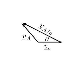
![\[ \ell \dot{\theta} = |\underline{\nu}_{A/o}|\]](https://engcourses-uofa.ca/wp-content/ql-cache/quicklatex.com-c0c0fcfc4381f3809cf4db835a56cf64_l3.png "Rendered by QuickLaTeX.com")
![\[ |\underline{\nu}_o| = \dot{x} \]](https://engcourses-uofa.ca/wp-content/ql-cache/quicklatex.com-cdb0335b2f6952781fac3cc4e63ed829_l3.png "Rendered by QuickLaTeX.com")
![\[ \begin{split} |\underline{\nu}_A| &= |\underline{\nu}_o|^2 + (\ell \dot{\theta})^2 - 2\nu_o\ell\dot{\theta}\cos\theta \\&= \dot{x}^2 + \frac{\ell^2}{r^2}\dot{x}^2 - 2\dot{x}^2\frac{\ell}{r} \cos \frac{x}{r} \end{split} \]](https://engcourses-uofa.ca/wp-content/ql-cache/quicklatex.com-7a933173744feec2922f60c14843a565_l3.png "Rendered by QuickLaTeX.com")
Thus:
![\[ T = \frac{\dot{x}^2}{2}\Big[\frac{3}{2}M + m\Big(1 + \frac{\ell^2}{r^2} - \frac{2\ell}{r}\cos\frac{x}{r}\Big)\Big] \]](https://engcourses-uofa.ca/wp-content/ql-cache/quicklatex.com-1b066805a2d75572b1f7622e83951149_l3.png "Rendered by QuickLaTeX.com")
![\[ V = mg\ell\Big(1-\cos\frac{x}{r}\Big) + \frac{1}{2}kx^2 \]](https://engcourses-uofa.ca/wp-content/ql-cache/quicklatex.com-1a86fe5996e67e1ddd80fca889d6cd1b_l3.png "Rendered by QuickLaTeX.com")
![\[\frac{\partial L}{\partial \dot{x}} = \dot{x}\Big[\frac{3M}{2} + m \Big(1+\frac{\ell^2}{r^2} - \frac{2\ell}{r}\cos\frac{x}{r}\Big)\Big] \]](https://engcourses-uofa.ca/wp-content/ql-cache/quicklatex.com-28e0f80ab1c81a8db846e391b3aca465_l3.png "Rendered by QuickLaTeX.com")
![\[\frac{\partial L}{\partial x} = \frac{\dot{x}^2}{2} \Big[ \frac{2\ell m}{r^2} \sin \frac{x}{r} \Big] -mg\frac{\ell}{r}\sin\frac{x}{r} - kx \]](https://engcourses-uofa.ca/wp-content/ql-cache/quicklatex.com-8a9f67e0dcd0fc00541d4ea684d96783_l3.png "Rendered by QuickLaTeX.com")
![\[ \frac{\text{d}}{\text{dt}}\Big(\frac{\partial L}{\partial \dot x}\Big) = \ddot{x}\Big[\frac{3M}{2} + m \Big( 1 + \frac{\ell^2}{r^2} - \frac{2\ell}{r}\cos\frac{x}{r} \Big)\Big] + \dot{x}^2\frac{2m\ell}{r^2}\sin\frac{x}{r} \]](https://engcourses-uofa.ca/wp-content/ql-cache/quicklatex.com-8ede3653db15f0bc27c2898262335a6c_l3.png "Rendered by QuickLaTeX.com")
The equation of motion comes from:
![\[ \frac{\text{d}}{\text{dt}} \Big(\frac{\partial L}{\partial \dot{x}}\Big) - \frac{\partial L}{\partial x} = -c\dot{x} \]](https://engcourses-uofa.ca/wp-content/ql-cache/quicklatex.com-90f11e4ed0d8376ad166c911bbae35ca_l3.png "Rendered by QuickLaTeX.com")
And becomes:
![\[ \Big[ \frac{3M}{2} + m \Big(1+ \frac{\ell^2}{r^2} - \frac{2\ell}{r}\cos\frac{x}{r}\Big)\Big]\ddot{x} + \dot{x}^2\frac{m\ell}{r^2}\sin{\frac{x}{r}} + mg\frac{\ell}{r}\sin{\frac{x}{r}} + kx + c\dot{x} = 0\]](https://engcourses-uofa.ca/wp-content/ql-cache/quicklatex.com-88a032617e6b2e0f0dff47a690090c33_l3.png "Rendered by QuickLaTeX.com")
For small deflection  and
and  :
:
![\[ \Big[\frac{3}{2}M + m\Big(1+\frac{\ell^2}{r^2}-\frac{2\ell}{r}\Big)\Big] \ddot{x} + \frac{m\ell x}{r^2}\Big[\frac{\dot{x}^2}{r}+g\Big] + kx + c\dot{x} = 0 \]](https://engcourses-uofa.ca/wp-content/ql-cache/quicklatex.com-4415740f93e680535871654756323774_l3.png "Rendered by QuickLaTeX.com")
![\[\left(\text{Set} \left(\frac{\dot{x}^2}{r}\right) \approx 0 \right)\]](https://engcourses-uofa.ca/wp-content/ql-cache/quicklatex.com-22903e2f61b4eef9b62dbc52f48ce06d_l3.png "Rendered by QuickLaTeX.com")
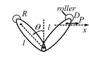
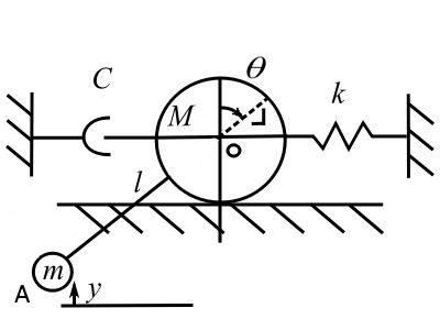
2 DOF Example
The uniform rod of length  and mass
  carries a slider of mass
  which is attached by a spring of stiffness
  . The spring is unstretched at
  .
.
![\[ T = \frac{1}{2}m_o\big[(r\dot{\theta})^2 + (\dot{r})^2\big] + \frac{1}{2}\Big(\frac{m\ell^2}{3}\dot{\theta}^2\Big) \]](https://engcourses-uofa.ca/wp-content/ql-cache/quicklatex.com-3d2725948e69ce2a60d0229080a0d843_l3.png "Rendered by QuickLaTeX.com")
![\[ V = \frac{1}{2}k(r-r_o)^2-m_ogr\cos\theta - mg\frac{\ell}{2}\cos\theta \]](https://engcourses-uofa.ca/wp-content/ql-cache/quicklatex.com-48035727c3f24c2913987e5a2b74c9e2_l3.png "Rendered by QuickLaTeX.com")
![\[L = T - V \quad \text{(} \theta = \frac{\pi}{2} \text{ is the datum)} \]](https://engcourses-uofa.ca/wp-content/ql-cache/quicklatex.com-e029dc3a0c0fc40154961316253be080_l3.png "Rendered by QuickLaTeX.com")
![\[\frac{\partial L}{\partial \dot{\theta}} = m_or^2\dot{\theta} + \frac{m\ell^2}{3}\dot{\theta} \]](https://engcourses-uofa.ca/wp-content/ql-cache/quicklatex.com-319c886402a413343f8ce07b74ae6039_l3.png "Rendered by QuickLaTeX.com")
![\[\frac{\partial L}{\partial \theta} = -m_ogr\sin \theta - mg\frac{\ell}{2}\sin\theta \]](https://engcourses-uofa.ca/wp-content/ql-cache/quicklatex.com-c64d9002eef22dc71ec59995e1dba7dd_l3.png "Rendered by QuickLaTeX.com")
![\[ \frac{\text{d}}{\text{dt}} \Big(\frac{\partial L}{\partial \dot{\theta}}\Big) - \frac{\partial L}{\partial \theta} = 0 \]](https://engcourses-uofa.ca/wp-content/ql-cache/quicklatex.com-dd4e06afe82ddb6da763d66e40b4043a_l3.png "Rendered by QuickLaTeX.com")
Thus:
![\[m_o r [r\ddot{\theta} + 2\dot{r}\dot{\theta}] + \frac{m\ell^2}{3}\dot{\theta} +m_ogr\sin\theta + mg\frac{\ell}{2}\sin\theta = 0 \]](https://engcourses-uofa.ca/wp-content/ql-cache/quicklatex.com-a7a5a20b344001f1d116af095bc7c269_l3.png "Rendered by QuickLaTeX.com")
Also, note that:
![\[ \frac{\partial L}{\partial \dot{r}} = m_o\dot{r} \]](https://engcourses-uofa.ca/wp-content/ql-cache/quicklatex.com-eb63a705c581932bd56655350cd98209_l3.png "Rendered by QuickLaTeX.com")
![\[ \frac{\partial L}{\partial r} = -k(r-r_o) + m_og\cos\theta + m_or\dot{\theta}^2 \]](https://engcourses-uofa.ca/wp-content/ql-cache/quicklatex.com-1270b2c90ae7c48a5b4f369270b18f75_l3.png "Rendered by QuickLaTeX.com")
![\[ \frac{\text{d}}{\text{dt}}\Big(\frac{\partial L}{\partial \dot{r}}\Big) - \frac{\partial L}{\partial r} = 0\]](https://engcourses-uofa.ca/wp-content/ql-cache/quicklatex.com-d10aad36c9a569b42c8b67afe69a64b9_l3.png "Rendered by QuickLaTeX.com")
Thus:
![\[ m_o\ddot{r} - m_or\dot{\theta}^2 + k(r-r_o) - m_og\cos\theta = 0\]](https://engcourses-uofa.ca/wp-content/ql-cache/quicklatex.com-c07940f99382d775e517631df810327b_l3.png "Rendered by QuickLaTeX.com")
The equilibrium positions are:
![\[\sin\theta = 0 \Rightarrow \theta = 0,\ \pi \]](https://engcourses-uofa.ca/wp-content/ql-cache/quicklatex.com-d8ccc08a2d607049467028e247343dce_l3.png "Rendered by QuickLaTeX.com")
![\[ k(r_\text{ST} - r_o) = \pm m_og \]](https://engcourses-uofa.ca/wp-content/ql-cache/quicklatex.com-5c8bd93be7c1abf928310e81565deca0_l3.png "Rendered by QuickLaTeX.com")
We could now study the stability of these configurations.
Example with External Forces
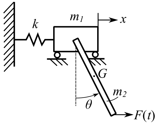
![\[ T = \frac{1}{2}m_1\dot{x}^2 + \frac{1}{2}m_2v_G^2 + \frac{1}{2}J_G\dot{\theta}^2 \]](https://engcourses-uofa.ca/wp-content/ql-cache/quicklatex.com-3d1e49d5b37525fb4310e87aae8357d9_l3.png "Rendered by QuickLaTeX.com")
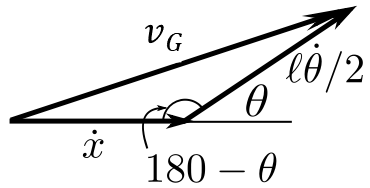
![\[ \nu_G^2 = \dot{x}^2 + \Big(\frac{\ell \dot{\theta}}{2}\Big)^2 - 2\dot{x}\Big(\frac{\ell\dot{\theta}}{2}\Big)\cos(180-\theta) \]](https://engcourses-uofa.ca/wp-content/ql-cache/quicklatex.com-1cc58e389a859336aa4af82c3e2cd635_l3.png "Rendered by QuickLaTeX.com")
Using  , we can say:
![\[ \begin{split} \cos(180-\theta) &= \cos 180 \cos \theta + \sin 180 \sin \theta \\& = -\cos \theta \end{split} \]](https://engcourses-uofa.ca/wp-content/ql-cache/quicklatex.com-e531cb81e00381697dd1b2375b7453f5_l3.png "Rendered by QuickLaTeX.com")
Thus:
![\[\nu_G^2 = \dot{x}^2 + \Big(\frac{\ell\dot{\theta}}{2}\Big)^2 + \dot{x}\ell\dot{\theta}\cos \theta \]](https://engcourses-uofa.ca/wp-content/ql-cache/quicklatex.com-33d701a368f25f2dc1a04de3ba69d97a_l3.png "Rendered by QuickLaTeX.com")
Therefore:
![\[T = \frac{1}{2}m_1\dot{x}^2 + \frac{1}{2}m_2\Big[\dot{x}^2 + \Big(\frac{\ell\dot{\theta}}{2}\Big)^2 + \dot{x}\dot{\theta}\ell\cos\theta \Big] + \frac{1}{2}J_G\dot{\theta}^2 \]](https://engcourses-uofa.ca/wp-content/ql-cache/quicklatex.com-bf3193bdba0a95ba1f3c0ea65394b5d9_l3.png "Rendered by QuickLaTeX.com")
![\[V = \frac{1}{2}kx^2 + m_2g\frac{\ell}{2}(1-\cos\theta) \]](https://engcourses-uofa.ca/wp-content/ql-cache/quicklatex.com-13dc79474710437adba4461c3a992e30_l3.png "Rendered by QuickLaTeX.com")
Where  is the datum. Now we must find the generalized forces. For a virtual displacement
  only:
only:
![\[ \delta W = F(t)\delta x \Rightarrow Q_x = F(t) \]](https://engcourses-uofa.ca/wp-content/ql-cache/quicklatex.com-f0462a061378e887a9ff038e85e72775_l3.png "Rendered by QuickLaTeX.com")
For a virtual displacement  only:
only:
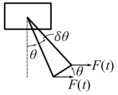
![\[ \delta W = \ell \delta \theta \cos\theta F(t) \]](https://engcourses-uofa.ca/wp-content/ql-cache/quicklatex.com-e14c5a8897f10337ffc0640efd0aa829_l3.png "Rendered by QuickLaTeX.com")
Therefore:
![\[ Q_\theta = F(t)\ell\cos\theta \]](https://engcourses-uofa.ca/wp-content/ql-cache/quicklatex.com-e3a90f151563eac2f627f1a4b252c85c_l3.png "Rendered by QuickLaTeX.com")
Then, note that:
![\[ \frac{\text{d}}{\text{dt}}\Big(\frac{\partial L}{\partial \dot{x}}\Big) - \frac{\partial L}{\partial x} = Q_x \quad (1) \]](https://engcourses-uofa.ca/wp-content/ql-cache/quicklatex.com-aa1c328c4395f7acb0752a3824e4968a_l3.png "Rendered by QuickLaTeX.com")
![\[ \frac{\text{d}}{\text{dt}} \Big(\frac{\partial L}{\partial \dot{\theta}}\Big) - \frac{\partial L}{\partial \theta} = Q_\theta \quad (2) \]](https://engcourses-uofa.ca/wp-content/ql-cache/quicklatex.com-47a33fcc597b780efa3b8c7071501b51_l3.png "Rendered by QuickLaTeX.com")
![\[ \frac{\partial L}{\partial \dot{x}} = m_1\dot{x} + m_2\dot{x} + m_2\frac{\ell}{2}\dot{\theta}\cos\theta \]](https://engcourses-uofa.ca/wp-content/ql-cache/quicklatex.com-2b32b2210a1b98478e8875d68a2dbeaa_l3.png "Rendered by QuickLaTeX.com")
![\[\frac{\partial L}{\partial x} = -kx\]](https://engcourses-uofa.ca/wp-content/ql-cache/quicklatex.com-7eb8d3f575847ccfb285aea4fae85c9e_l3.png "Rendered by QuickLaTeX.com")
![\[ \frac{\partial L}{\partial \dot{\theta}} = m_2\frac{\ell^2}{4}\dot{\theta} + m_2\dot{x}\frac{\ell}{2}\cos\theta + J_G\dot{\theta} \]](https://engcourses-uofa.ca/wp-content/ql-cache/quicklatex.com-3e65b2085830f2cc95c49e19d5e57bee_l3.png "Rendered by QuickLaTeX.com")
![\[ \frac{\partial L}{\partial \theta} = -\frac{m_2}{2}\dot{x}\dot{\theta}\ell\sin\theta - m_2g\frac{\ell}{2}\sin\theta \]](https://engcourses-uofa.ca/wp-content/ql-cache/quicklatex.com-8461ad1110700feeec0b51a832d4f1f8_l3.png "Rendered by QuickLaTeX.com")
Therefore, (1) becomes:
![\[ m_1\ddot{x} + m_2\ddot{x} + m_2\frac{\ell}{2}[\ddot{\theta}\cos\theta - \dot{\theta}^2\sin\theta]+kx = F(t) \]](https://engcourses-uofa.ca/wp-content/ql-cache/quicklatex.com-1f523d132907cf59bb8eb35c4d5a5f43_l3.png "Rendered by QuickLaTeX.com")
And (2) becomes:
![\[m_2 \frac{\ell^2}{4}\ddot{\theta} + m_2\ddot{x}\frac{\ell}{2}\cos\theta - m_2\dot{x}\frac{\ell}{2}\dot{\theta}\sin\theta + \frac{1}{12}m\ell^2\ddot{\theta} + m_2\dot{x}\frac{\ell}{2}\dot{\theta}\sin\theta + m_2g\frac{\ell}{2}\sin\theta = F(t)\ell\cos\theta \]](https://engcourses-uofa.ca/wp-content/ql-cache/quicklatex.com-bec62bcdc89739c25a58d6853ba0f0e5_l3.png "Rendered by QuickLaTeX.com")
![\[ m_2\frac{\ell^2}{3}\ddot{\theta} + \frac{m_2}{2}\ddot{x}\ell\cos\theta + m_2g\frac{\ell}{2}\sin\theta = F(t)\ell\cos\theta \]](https://engcourses-uofa.ca/wp-content/ql-cache/quicklatex.com-cae9832ab51b770a69992b5bdb28782b_l3.png "Rendered by QuickLaTeX.com")
For small angles these become:
![\[ (m_1+m_2)\ddot{x} + m_2\frac{\ell}{2}\ddot{\theta} + kx = F(t) \]](https://engcourses-uofa.ca/wp-content/ql-cache/quicklatex.com-1a44b4f392f5cbde7a79db7a449de901_l3.png "Rendered by QuickLaTeX.com")
![\[ m_2\frac{\ell^2}{3}\ddot{\theta} + m_2\frac{\ell}{2}\ddot{x} + m_2g\frac{\ell}{2}\theta = F(t)\ell \]](https://engcourses-uofa.ca/wp-content/ql-cache/quicklatex.com-1bd4424ffe0385afc5d7107445b182cd_l3.png "Rendered by QuickLaTeX.com")
If we have support motion instead of forcing,
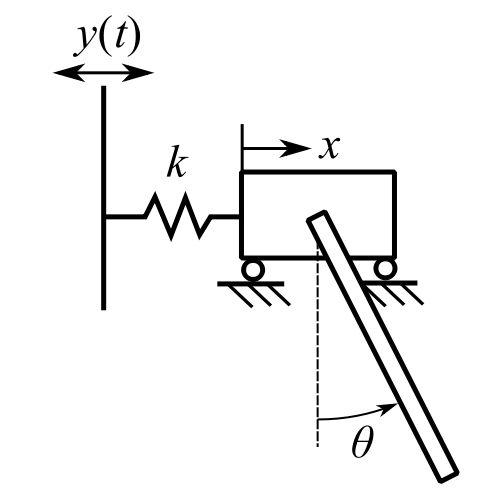
then we cannot neccesairly use a potential, so now give the system a and . For a :
![\[ \delta W = -k(x-y)\delta x \]](https://engcourses-uofa.ca/wp-content/ql-cache/quicklatex.com-3c212ade73370589238234f4f03f2ff4_l3.png "Rendered by QuickLaTeX.com")
Therefore:
![\[Q_x = -k(x-y) \]](https://engcourses-uofa.ca/wp-content/ql-cache/quicklatex.com-a3f3ad880a5496da23351b95820400b4_l3.png "Rendered by QuickLaTeX.com")
![\[Q_\theta = 0 \]](https://engcourses-uofa.ca/wp-content/ql-cache/quicklatex.com-04a5ec5c7b4bc87a7d6f2559169c8075_l3.png "Rendered by QuickLaTeX.com")
 as no work is done for alone. Thus, is the same, and:
![\[ V = m_2g\frac{\ell}{2}(1-\cos\theta) \]](https://engcourses-uofa.ca/wp-content/ql-cache/quicklatex.com-9c42c08a36a54b0b86037bbf344b57d8_l3.png "Rendered by QuickLaTeX.com")
For small motions:
![\[ (m_1+m_2)\ddot{x} +m_2\frac{\ell}{2}\ddot{\theta} + kx = ky(t) \]](https://engcourses-uofa.ca/wp-content/ql-cache/quicklatex.com-5b7a75461f02cccb17c3f968ba5884a4_l3.png "Rendered by QuickLaTeX.com")
![\[ m_2\frac{\ell^2}{3} \ddot{\theta} + m_2\frac{\ell}{2}\ddot{x} + m_2g\frac{\ell}{2}\theta = 0\]](https://engcourses-uofa.ca/wp-content/ql-cache/quicklatex.com-3889293806561789ec6e7dd468b2659c_l3.png "Rendered by QuickLaTeX.com")
Thus:
![\[ \begin{bmatrix} m_1 + m_2 & m_2\frac{\ell}{2} \\ m_2\frac{\ell}{2} & m_2\frac{\ell^2}{3} \end{bmatrix} \begin{Bmatrix} \ddot{x} \\ \ddot{\theta} \end{Bmatrix} + \begin{bmatrix} k & 0 \\ 0 & \frac{m_2g\ell}{2} \end{bmatrix} \begin{Bmatrix} x \\ \theta \end{Bmatrix} = \begin{Bmatrix} ky(t) \\ 0 \end{Bmatrix} \]](https://engcourses-uofa.ca/wp-content/ql-cache/quicklatex.com-093b8b0d2267ec5448c3ea3ff423a3a8_l3.png "Rendered by QuickLaTeX.com")
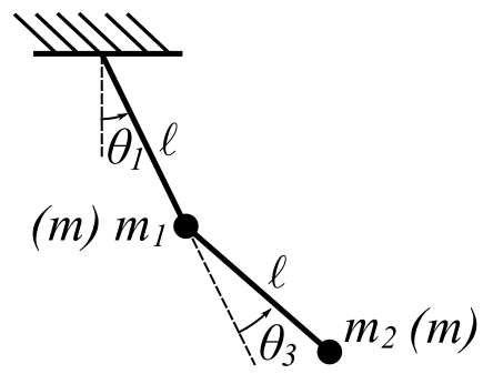
Example
Consider the double pendulum:
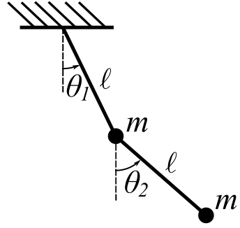
![\[T = \frac{1}{2}m(\ell\dot{\theta_1})^2 + \frac{1}{2}m(\ell\dot{\theta_1} + \ell\dot{\theta_2})^2 \]](https://engcourses-uofa.ca/wp-content/ql-cache/quicklatex.com-fffb753af24093f3ab659ea5a7958034_l3.png "Rendered by QuickLaTeX.com")
![\[V = mg\ell(1-\cos\theta_1) + mg\ell(1 - \cos\theta_1 + 1-\cos\theta_2) \]](https://engcourses-uofa.ca/wp-content/ql-cache/quicklatex.com-dd4e4b91b2f9b518e404db5c0a2e8755_l3.png "Rendered by QuickLaTeX.com")
Consider only small angles. Thus:
![\[ V \approx mg\ell\frac{\theta_1^2}{2} + mg\ell\Big(\frac{\theta_1^2}{2} + \frac{\theta_2^2}{2}\Big) \]](https://engcourses-uofa.ca/wp-content/ql-cache/quicklatex.com-b13b7f87844bf86381b0705421a6bae0_l3.png "Rendered by QuickLaTeX.com")
Then:
![\[ \frac{\partial L}{\partial \dot{\theta_1}} = m\ell^2\dot{\theta_1} + m\ell^2(\dot{\theta_1} + \dot{\theta_2}) \]](https://engcourses-uofa.ca/wp-content/ql-cache/quicklatex.com-9a33c2905e3fea05901edd4c8652c0af_l3.png "Rendered by QuickLaTeX.com")
![\[ \frac{\partial L}{\partial \dot{\theta_2}} = m\ell^2(\dot{\theta_1} + \dot{\theta_2}) \]](https://engcourses-uofa.ca/wp-content/ql-cache/quicklatex.com-f8a03034d68402ba0eee244094013247_l3.png "Rendered by QuickLaTeX.com")
![\[ \frac{\partial L}{\partial \theta_1} = -mg\ell\theta_1 - mg\ell\theta_1 \]](https://engcourses-uofa.ca/wp-content/ql-cache/quicklatex.com-9cb3ed566d90561e600f20084786fbe3_l3.png "Rendered by QuickLaTeX.com")
![\[ \frac{\partial L}{\partial \theta_2} = -mg\ell\theta_2 \]](https://engcourses-uofa.ca/wp-content/ql-cache/quicklatex.com-f7d9f0195c5feeacd6ab8424bd9ed1d7_l3.png "Rendered by QuickLaTeX.com")
Therefore:
![\[ \begin{bmatrix} 2 & 1 \\ 1 & 1 \end{bmatrix} \begin{Bmatrix} \ddot{\theta_1} \\ \ddot{\theta_2} \end{Bmatrix} + \frac{g}{\ell} \begin{bmatrix} 2 & 0 \\ 0 & 1 \end{bmatrix} \begin{Bmatrix} \theta_1 \\ \theta_2 \end{Bmatrix} = \begin{Bmatrix} 0 \\ 0 \end{Bmatrix} \]](https://engcourses-uofa.ca/wp-content/ql-cache/quicklatex.com-305ab3b832409cd2cfda64b3c4c66dcb_l3.png "Rendered by QuickLaTeX.com")
![\[ [m]^{-1} = \begin{bmatrix} 1 & -1 \\ -1 & 2 \end{bmatrix} \]](https://engcourses-uofa.ca/wp-content/ql-cache/quicklatex.com-0df66432fd2d0044f2a10e00d5b2dba1_l3.png "Rendered by QuickLaTeX.com")
![\[\begin{split} [m]^{-1}[m] &= \begin{bmatrix} 1 & -1 \\ -1 & 2 \end{bmatrix} \begin{bmatrix} 2 & 1 \\ 1 & 1 \end{bmatrix} \\&= \begin{bmatrix} 1 & 0 \\ 0 & 1 \end{bmatrix} \end{split}\]](https://engcourses-uofa.ca/wp-content/ql-cache/quicklatex.com-fb3b703ad19acc1e0e28d03524f57239_l3.png "Rendered by QuickLaTeX.com")
![\[ -p^2\begin{Bmatrix} X_1 \\ X_2 \end{Bmatrix} + \frac{g}{\ell}\begin{bmatrix} 1 & -1 \\ -1 & 2 \end{bmatrix} \begin{bmatrix} 2 & 0 \\ 0 & 1 \end{bmatrix} \begin{Bmatrix} X_1 \\ X_2 \end{Bmatrix} = 0 \]](https://engcourses-uofa.ca/wp-content/ql-cache/quicklatex.com-525938664c229a705509903d4f3a126b_l3.png "Rendered by QuickLaTeX.com")
![\[ \implies -\frac{p^2\ell}{g} \begin{Bmatrix} X_1 \\ X_2 \end{Bmatrix} + \begin{bmatrix} 2 & -1 \\ -2 & 2 \end{bmatrix} \begin{Bmatrix} X_1 \\ X_2\end{Bmatrix} = 0\]](https://engcourses-uofa.ca/wp-content/ql-cache/quicklatex.com-e8741bac746d820b5e3508e05907f9b6_l3.png "Rendered by QuickLaTeX.com")
Set  :
:
![\[ \begin{vmatrix} 2 - \lambda^2 & -1 \\ -2 & 2 - \lambda^2 \end{vmatrix} = 0\]](https://engcourses-uofa.ca/wp-content/ql-cache/quicklatex.com-1e1b243f70df120f5ec3d5d51c3fefe9_l3.png "Rendered by QuickLaTeX.com")
![\[ (2 - \lambda ^2 ) ^2 - 2 = 0 \]](https://engcourses-uofa.ca/wp-content/ql-cache/quicklatex.com-4ba2206428189f6cba4dafab0821d3a4_l3.png "Rendered by QuickLaTeX.com")
![\[ 4 - 4\lambda^2 + \lambda^4 - 2 = 0\]](https://engcourses-uofa.ca/wp-content/ql-cache/quicklatex.com-c6bccf0b1ba52cd67873391518fa5c25_l3.png "Rendered by QuickLaTeX.com")
![\[\lambda^4 - 4\lambda^2 + 2 = 0 \]](https://engcourses-uofa.ca/wp-content/ql-cache/quicklatex.com-ea5fa5d756a3e8e508d9fa1c80d9eb4f_l3.png "Rendered by QuickLaTeX.com")
![\[ \lambda^2 = 2 \pm \sqrt{2} \]](https://engcourses-uofa.ca/wp-content/ql-cache/quicklatex.com-3d33269d8321532b5d808c52e034d949_l3.png "Rendered by QuickLaTeX.com")
![\[ (2-\lambda^2)X_1 - X_2 = 0\]](https://engcourses-uofa.ca/wp-content/ql-cache/quicklatex.com-fb1a1255c8c4f82e276bab464c04332d_l3.png "Rendered by QuickLaTeX.com")
![\[ \frac{X_2}{X_1} = 2 - \lambda^2\]](https://engcourses-uofa.ca/wp-content/ql-cache/quicklatex.com-215a38ba3ecb394207055990c50dba7a_l3.png "Rendered by QuickLaTeX.com")
![\[ \bigg(\frac{X_2}{X_1}\bigg)_1 = 2 - 2 + \sqrt{2} = \underline{\underline{\sqrt{2}}} \]](https://engcourses-uofa.ca/wp-content/ql-cache/quicklatex.com-204818e0646df2bdd2d3070623d9f258_l3.png "Rendered by QuickLaTeX.com")
![\[ \bigg(\frac{X_2}{X_1}\bigg)_1 = 2 - 2 - \sqrt{2} = \underline{\underline{-\sqrt{2}}} \]](https://engcourses-uofa.ca/wp-content/ql-cache/quicklatex.com-14e0a34771e277f8cf29be9ce421d8eb_l3.png "Rendered by QuickLaTeX.com")
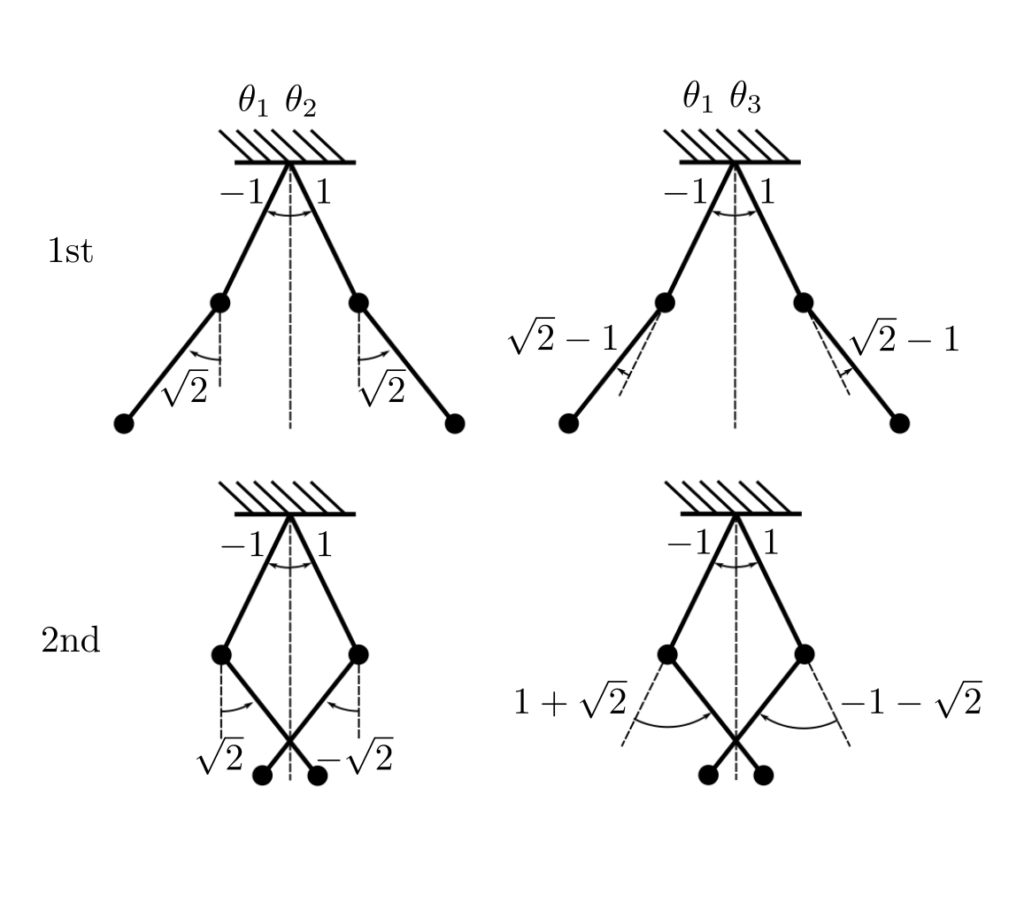
Example
Now try a different set of generalized coordinates for the same problem.
If we consider small angles:
![\[ T = \frac{1}{2} m(\ell \dot{\theta}_1)^2 + \frac{1}{2}m\big[\ell\dot{\theta}_1 + \ell(\dot{\theta}_1+ \dot{\theta}_3)\big]^2 \]](https://engcourses-uofa.ca/wp-content/ql-cache/quicklatex.com-76a3f3bf7fa0962c01a5029a57ab83d9_l3.png "Rendered by QuickLaTeX.com")
![\[ V = mg\ell(1-\cos{\theta_1}) + mg\ell\big[ 1-\cos{\theta_1} + 1 - \cos{(\theta_1 + \theta_3)}\big] \]](https://engcourses-uofa.ca/wp-content/ql-cache/quicklatex.com-83df0fd8d7bfb305ab7264855e6eb45a_l3.png "Rendered by QuickLaTeX.com")
Therefore:
![\[V = -mg\ell\frac{\theta_1^2}{2} - mg\ell\bigg[ \frac{\theta_1^2}{2} + \frac{(\theta_2 + \theta_3)^2}{2} \bigg] \]](https://engcourses-uofa.ca/wp-content/ql-cache/quicklatex.com-e3527d46cc9da73e7efabc9119b6731d_l3.png "Rendered by QuickLaTeX.com")
![\[T = \frac{1}{2}m\ell^2(\dot{\theta}_1)^2 + \frac{1}{2}m\ell^2[2\dot{\theta}_1+\dot{\theta}_3]^2\]](https://engcourses-uofa.ca/wp-content/ql-cache/quicklatex.com-3eb92b1af391e9dac0834d9df5873736_l3.png "Rendered by QuickLaTeX.com")
![\[V = -mg\ell\theta_1^2-mg\frac{\ell}{2}(\theta_1 +\theta_3)^2 \]](https://engcourses-uofa.ca/wp-content/ql-cache/quicklatex.com-d2917487e681f68b5cf74f4b3c9494ab_l3.png "Rendered by QuickLaTeX.com")
![\[L = T-V\]](https://engcourses-uofa.ca/wp-content/ql-cache/quicklatex.com-f50d738788ac2af2edff52c2b11eea23_l3.png "Rendered by QuickLaTeX.com")
![\[\begin{split}\frac{\partial L}{\partial \dot\theta_1} &= m\ell^2\dot\theta_1 +\frac{1}{2}m\ell^22(2\dot\theta_1+\dot\theta_3)2 \\&= m\ell^2[5\dot\theta_1 + 2\dot\theta_3]\end{split}\]](https://engcourses-uofa.ca/wp-content/ql-cache/quicklatex.com-a7a5152ed01fc147056e7fa7633f4c55_l3.png "Rendered by QuickLaTeX.com")
![\[\begin{split}\frac{\partial L}{\partial \dot\theta_3} &= \frac{1}{2}m\ell^2(2)[2\dot\theta_1+\dot\theta_3] \\&= m\ell^2[2\dot\theta_1+\dot\theta_3]\end{split}\]](https://engcourses-uofa.ca/wp-content/ql-cache/quicklatex.com-f22028c92ff679d646ff7c11963112bb_l3.png "Rendered by QuickLaTeX.com")
![\[\frac{\partial L}{\partial \theta_1 } = -2mg\ell\theta_1 - mg\ell(\theta_1+\theta_3)\]](https://engcourses-uofa.ca/wp-content/ql-cache/quicklatex.com-eca3bca25be94e3ba168d0d9e750b56a_l3.png "Rendered by QuickLaTeX.com")
![\[\frac{\partial L}{\partial \theta_3} = -mg\ell(\theta_1 +\theta_3)\]](https://engcourses-uofa.ca/wp-content/ql-cache/quicklatex.com-de09f4c47dfcc962cce092d16a17f7d0_l3.png "Rendered by QuickLaTeX.com")
![\[\frac{d}{dt}\bigg(\frac{\partial L}{\partial \dot\theta_1}\bigg) - \frac{\partial L}{\partial \theta_1} = 0\]](https://engcourses-uofa.ca/wp-content/ql-cache/quicklatex.com-68304399c23384398111eaa19996598f_l3.png "Rendered by QuickLaTeX.com")
![\[ m\ell^2[5\ddot\theta_1 + 2 \ddot\theta_3] +3mg\ell\theta_1 + mg\ell\theta_3 = 0\]](https://engcourses-uofa.ca/wp-content/ql-cache/quicklatex.com-e10564a2fc9aec4798ee9154200c9206_l3.png "Rendered by QuickLaTeX.com")
![\[m\ell^2[2\ddot\theta_1 + \ddot\theta_3] + mg\ell(\theta_1 + \theta_3) = 0\]](https://engcourses-uofa.ca/wp-content/ql-cache/quicklatex.com-6997bf21a4594169d0cb36dc7d3841ba_l3.png "Rendered by QuickLaTeX.com")
Therefore:
![\[\begin{bmatrix} 5 & 2 \\ 2 & 1 \end{bmatrix}\begin{Bmatrix} \ddot\theta_1 \\ \ddot\theta_3 \end{Bmatrix} + \frac{g}{\ell}\begin{bmatrix} 3 & 1 \\ 1 & 1 \end{bmatrix}\begin{Bmatrix} \theta_1 \\ \theta_2 \end{Bmatrix} = \begin{Bmatrix} 0 \\ 0 \end{Bmatrix} \]](https://engcourses-uofa.ca/wp-content/ql-cache/quicklatex.com-1d92a9add494f68c1d6135d50a9f8c0e_l3.png "Rendered by QuickLaTeX.com")
Therefore:
![\[ - \frac{p^2\ell}{g}\begin{bmatrix} 5 & 2 \\ 2 & 1 \end{bmatrix}\begin{Bmatrix} X_1 \\ X_2\end{Bmatrix} + \begin{bmatrix} 3 & 1 \\ 1 & 1 \end{bmatrix} \begin{Bmatrix} X _1 \\ X_2 \end{Bmatrix} = \begin{Bmatrix} 0 \\ 0 \end{Bmatrix} \]](https://engcourses-uofa.ca/wp-content/ql-cache/quicklatex.com-c08adf3ad5d7a869b5a4c46e29f82f11_l3.png "Rendered by QuickLaTeX.com")
![\[ [m]^{-1}[m] = \begin{bmatrix} 1 & -2 \\ -2 & 5 \end{bmatrix} \begin{bmatrix} 5 & 2 \\ 2 & 1 \end{bmatrix} = \begin{bmatrix} 1 & 0 \\ 0 & 1 \end{bmatrix} \]](https://engcourses-uofa.ca/wp-content/ql-cache/quicklatex.com-18cad55b725e11117d4b0125cbcb3264_l3.png "Rendered by QuickLaTeX.com")
Set :
![\[ -\lambda^2\begin{Bmatrix} X_1 \\ X_3 \end{Bmatrix} + \begin{bmatrix} 1 & -2 \\ -2 & 5 \end{bmatrix} \begin{bmatrix} 3 & 1 \\ 1 & 1 \end{bmatrix} \begin{Bmatrix} X_1 \\ X_3 \end{Bmatrix} = \begin{Bmatrix} 0 \\ 0 \end{Bmatrix} \]](https://engcourses-uofa.ca/wp-content/ql-cache/quicklatex.com-0db765620d2b996481d655baf4d2f084_l3.png "Rendered by QuickLaTeX.com")
![\[ -\lambda^2\begin{Bmatrix} X_1 \\ X_3 \end{Bmatrix} + \begin{bmatrix} 1 & -1 \\ -1 & 3 \end{bmatrix} \begin{Bmatrix} X-1 \\ X_3 \end{Bmatrix} = \begin{Bmatrix} 0 \\ 0 \end{Bmatrix} \]](https://engcourses-uofa.ca/wp-content/ql-cache/quicklatex.com-f63f0c170dc3d1273bddfe4c8d46e966_l3.png "Rendered by QuickLaTeX.com")
Therefore:
![\[ (1 - \lambda^2)(3 - \lambda^2) - 1 = 0 \]](https://engcourses-uofa.ca/wp-content/ql-cache/quicklatex.com-28621b05a38e6de96aa3ffa3fa573285_l3.png "Rendered by QuickLaTeX.com")
![\[\lambda^4 - 4\lambda^2 + 2 = 0 \quad \text{(same characteristic equation)}\]](https://engcourses-uofa.ca/wp-content/ql-cache/quicklatex.com-dcee5789257136e765b99e40735d302d_l3.png "Rendered by QuickLaTeX.com")
Therefore:
For mode shapes:
![\[ (1 - \lambda^2) X_1 - X_3 = 0 \]](https://engcourses-uofa.ca/wp-content/ql-cache/quicklatex.com-19848acfccb9fd97b53b442bbbbfee32_l3.png "Rendered by QuickLaTeX.com")
![\[ \implies \frac{X_3}{X_1} = 1 - \lambda^2 \]](https://engcourses-uofa.ca/wp-content/ql-cache/quicklatex.com-6e4ea415c29d50d572c46c978c76a392_l3.png "Rendered by QuickLaTeX.com")
![\[\begin{split} \bigg(\frac{X_3}{X_1}\bigg)_1 &= 1 - 2 + \sqrt{2} \\&= -1 + \sqrt{2} \end{split}\]](https://engcourses-uofa.ca/wp-content/ql-cache/quicklatex.com-e7ecc506c117df697a5451682804041d_l3.png "Rendered by QuickLaTeX.com")
![\[\begin{split} \bigg(\frac{X_3}{X_1} \bigg) _2 &= 1 - 2 - \sqrt{2} \\&= -1 - \sqrt{2} \end{split}\]](https://engcourses-uofa.ca/wp-content/ql-cache/quicklatex.com-4e2c09dffd8471e01f72e9c1124af2af_l3.png "Rendered by QuickLaTeX.com")
These are different values of ratios than in the first case. However, when plotted:
Now use the newtonain approach to the same problem:
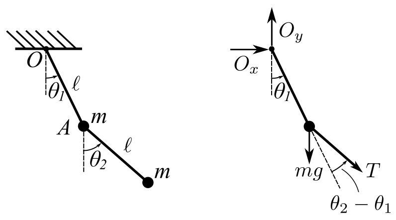
![\[ +\circlearrowleft \sum M_0 = m\ell\ddot\theta_1 = - mg\ell\theta_1 + T( \theta_2 - \theta_1) \ell \quad \text{(A)} \]](https://engcourses-uofa.ca/wp-content/ql-cache/quicklatex.com-038511a62cd7fb292c8402a4512f2f0a_l3.png "Rendered by QuickLaTeX.com")
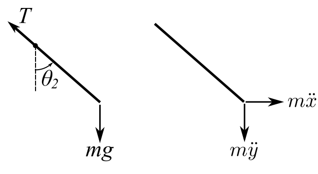
![\[\begin{split} + \downarrow \sum F_y &= m\ddot y \\&= -T\cos\theta_2 + mg \end{split}\]](https://engcourses-uofa.ca/wp-content/ql-cache/quicklatex.com-9e83e2224a85739e04670d16fbd11438_l3.png "Rendered by QuickLaTeX.com")
![\[\begin{split} + \rightarrow \sum F_x &= m\ddot x \\&= - T\sin{\theta_2} \end{split}\]](https://engcourses-uofa.ca/wp-content/ql-cache/quicklatex.com-e535fdd82e3b963fd92f6d124f774b5b_l3.png "Rendered by QuickLaTeX.com")
![\[\ddot{x} \approx \ell ( \ddot\theta_1 + \ddot\theta_2) , \ \ddot y \approx 0 \]](https://engcourses-uofa.ca/wp-content/ql-cache/quicklatex.com-0842df6d9307b974c3d6e98f38efadd5_l3.png "Rendered by QuickLaTeX.com")
Therefore:
![\[T \approx mg \]](https://engcourses-uofa.ca/wp-content/ql-cache/quicklatex.com-0ded86ea773436105d87f5a680f23a40_l3.png "Rendered by QuickLaTeX.com")
![\[ m\ell(\ddot\theta_1 + \ddot\theta_2) + mg\theta_2 = 0 \quad \text{(B)}\]](https://engcourses-uofa.ca/wp-content/ql-cache/quicklatex.com-68871b387b4984240ac4b7cd56da6f33_l3.png "Rendered by QuickLaTeX.com")
![\[\begin{bmatrix} m\ell & 0 \\ m\ell & m\ell \end{bmatrix} \begin{Bmatrix} \ddot\theta_1 \\ \ddot\theta_2 \end{Bmatrix} + \begin{bmatrix} 2mg & -mg \\ 0 & mg \end{bmatrix} \begin{Bmatrix} \theta_1 \\ \theta_2 \end{Bmatrix} = \begin{Bmatrix} 0 \\ 0 \end{Bmatrix} \]](https://engcourses-uofa.ca/wp-content/ql-cache/quicklatex.com-aaa3923ec449de3107aefc4aa15e39c9_l3.png "Rendered by QuickLaTeX.com")
Note both mass and stiffness matrices are non-symmetric!
Calculating the eigenvalues gives the same result and the mode shapes are identical with the other 2 formulations.
NOTE: These sets (first and third formulation) are linearly dependent.
Lagrange’s Equation for Small Oscillations
Our main interest is in the motion of MDOF systems in the neighborhood of equilibrium positions. WLOG we assume the equilibrium position is  and that the displacements are sufficiently small that the linear force- displacement and force-velocity relations hold. This means that the generalized coordinates and their time derivatives appear in the differential equations to only the first power.
Therefore:
![\[ \underline{\dot r} = \sum_{k = 1}^n \frac{\partial \underline{r}}{\partial q_k}\dot{q}_k \]](https://engcourses-uofa.ca/wp-content/ql-cache/quicklatex.com-60bc49680291cfbec6e1a9d45175b2c3_l3.png "Rendered by QuickLaTeX.com")
And  are constants.
![\[\begin{split} T &= \frac{1}{2} \sum_{i = 1}^N m_i \underline{\dot r}_i \underline{\dot r}_i \\&= \frac{1}{2} \sum_{i = 1}^N m_i\bigg(\sum_{r = 1}^n \frac{\partial \underline{r}_i}{\partial q_r}\dot{q}_r\bigg)\bigg(\sum_{s = 1}^n \frac{\partial \underline{r}_i}{\partial q_s}\dot{q}_s\bigg) \\&= \frac{1}{2} \sum_{r = 1}^n \sum_{s = 1}^n\bigg(\sum_{i=1}^N m_i \frac{\partial \underline{r}_i}{\partial q_r}\frac{\partial \underline{r}_i}{\partial q_s}\bigg)\dot q_r\dot q_s \end{split}\]](https://engcourses-uofa.ca/wp-content/ql-cache/quicklatex.com-9d1e0ae2b0af985b5c3a8f28d0d3bbe4_l3.png "Rendered by QuickLaTeX.com")
Set  as the generalized masses.
Similarly we can write the potential energy as  and consider a Taylor expansion of V about the equilibrium configuration.
![\[V(q_n) = V_0 \sum_{n = 1} ^n \frac{\partial V}{\partial q_i} + \frac{1}{2}\sum_{i= 1}^n \sum_{j = 1}^n \frac{\partial^2V}{\partial q_i \partial q_j}q_iq_j+ \dotsc\]](https://engcourses-uofa.ca/wp-content/ql-cache/quicklatex.com-6da3dab0113b216fde230aca11f8c191_l3.png "Rendered by QuickLaTeX.com")
Where the partial derivatives are all evaluated at  .
.
As the equilibrium point is a condition in which:
![\[\frac{\partial V}{\partial q_i} = 0\]](https://engcourses-uofa.ca/wp-content/ql-cache/quicklatex.com-f4fb8ffa8f4aaf338dc6b79a51f640d0_l3.png "Rendered by QuickLaTeX.com")
is approximately:
![\[\begin{split} V &= \frac{1}{2}\sum_{r = 1}^n \sum_{s = 1}^n \frac{\partial^2 V}{\partial q_r \partial q_s}q_rq_s \\&=\frac{1}{2}\sum_{r = 1}^n \sum_{s = 1}^n k_{rs}q_rq_s\end{split}\]](https://engcourses-uofa.ca/wp-content/ql-cache/quicklatex.com-2f3793ee67b0daf2d4a33e358acd59ca_l3.png "Rendered by QuickLaTeX.com")
Where  are the stiffness coefficients. If we now use Lagrange’s equation the equations of motion become:
![\[\frac{\partial L}{\partial \dot{q}_j} = \sum_{s = 1}^n m_{js}\dot{q}_s \]](https://engcourses-uofa.ca/wp-content/ql-cache/quicklatex.com-fb76e1e347dc559fc846ecda209ff06d_l3.png "Rendered by QuickLaTeX.com")
![\[\frac{\partial L}{\partial q_j} = \sum_{s = 1}^n k_{js}q_s \]](https://engcourses-uofa.ca/wp-content/ql-cache/quicklatex.com-a041be2fa2387bb9b69a5eaa697c337c_l3.png "Rendered by QuickLaTeX.com")
Therefore
![\[\sum_{s = 1}^n[m_{js} \ddot{q}_s(t) + k_{js}q(t)] = Q_j \]](https://engcourses-uofa.ca/wp-content/ql-cache/quicklatex.com-43355662605c9e5edbcdb08432974007_l3.png "Rendered by QuickLaTeX.com")
![\[j = 1,2 \dotsc n\]](https://engcourses-uofa.ca/wp-content/ql-cache/quicklatex.com-d70e6fa6dd38ea195580a1a3ddfee913_l3.png "Rendered by QuickLaTeX.com")
While this is very straightforward, we can use this result to obtain approximate formulations of the equations of motion as continuous systems it replaces them with a  degree of freedom system. It can also extend the technique to find approximate response to a specific forcing function. This is called the assumed modes method (AMM).
For discrete system it replaces them with a smaller number of DOF, while for continuous system it replaces them with an degree of freedom system. We can also easily extend it to a forced system.
Then the method assumes:
![\[y(x,t) = \sum_{i = 1}^N\phi_iq_i(t) \]](https://engcourses-uofa.ca/wp-content/ql-cache/quicklatex.com-6a3b9dc058662f3211716857fa8e9889_l3.png "Rendered by QuickLaTeX.com")
Where  are trial functions and
  are the generalized coordinates.
![\[ T = \frac{1}{2}\sum_{i=1}^N\sum_{j=1}^Nm_{ij}\dot{q}_i\dot{q}_j\]](https://engcourses-uofa.ca/wp-content/ql-cache/quicklatex.com-078ab4dfe534a0813de345e47fde7d43_l3.png "Rendered by QuickLaTeX.com")
![\[V = \frac{1}{2}\sum_{i = 1}^N\sum_{j = 1}^Nk_{ij}q_iq_j\]](https://engcourses-uofa.ca/wp-content/ql-cache/quicklatex.com-170fac38709a00e7ff1fc3c6174a9bf0_l3.png "Rendered by QuickLaTeX.com")
needs only satisfy the geometric boundary conditions.
For continuous systems:
![\[\begin{split}T &= \frac{1}{2} \int dm\bigg(\frac{\partial y}{\partial t}\bigg)^2 \\&= \frac{1}{2} \sum_{i = 1}^N\sum_{j = 1}^N\dot{q}_i\dot{q}_j\int_m \phi_i(x)\phi_j(x)dm\end{split} \]](https://engcourses-uofa.ca/wp-content/ql-cache/quicklatex.com-82cd882cdf659ac281bf1df5e97f63f3_l3.png "Rendered by QuickLaTeX.com")
Therefore:
![\[m_{ij} = \int_m \phi_i(x)\phi_j(x)dm \]](https://engcourses-uofa.ca/wp-content/ql-cache/quicklatex.com-27deb34414bb16376639cbdd767b53b4_l3.png "Rendered by QuickLaTeX.com")
While for discrete systems
![\[ m_{ij} = \sum_{p = 1}^N m_p\phi_i(x_p)\phi_j(x_p)\]](https://engcourses-uofa.ca/wp-content/ql-cache/quicklatex.com-f05d5300cf47eff09325336373232fd9_l3.png "Rendered by QuickLaTeX.com")
The potential energy can be determined is a similar manner.
Consider a generalized beam:
![\[ V = \frac{1}{2}\int_m EI \frac{\partial^2 y}{\partial x^2}dx \]](https://engcourses-uofa.ca/wp-content/ql-cache/quicklatex.com-8e916a591456d7e75641de141b77df0b_l3.png "Rendered by QuickLaTeX.com")
![\[\frac{\partial^2 y}{\partial x^2} = \sum_{i=1}^N \phi''(x)(t)\]](https://engcourses-uofa.ca/wp-content/ql-cache/quicklatex.com-7059793a4cf1eb0c1c506ae20432c880_l3.png "Rendered by QuickLaTeX.com")
Therefore:
![\[ V = \frac{1}{2}\sum_{i = 1}^N\sum_{j=1}^Nq_iq_j\int_LEI\phi''_i\phi''_jdx\]](https://engcourses-uofa.ca/wp-content/ql-cache/quicklatex.com-acb8ee71350250f0a17beea4263aafd6_l3.png "Rendered by QuickLaTeX.com")
![\[k_{ij} = \int EI\phi''_i\phi''_jdx\]](https://engcourses-uofa.ca/wp-content/ql-cache/quicklatex.com-c7f1bd2441745dca34514fe2f8f42bf0_l3.png "Rendered by QuickLaTeX.com")
This will allow calculation of a consistent mass and stiffness matrices.
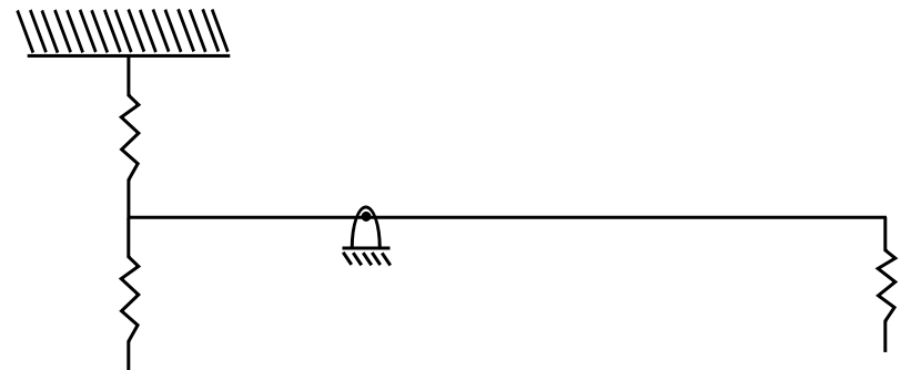
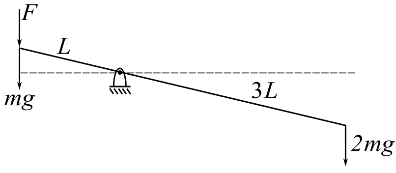
Example: Discrete System

![\[m_1 = m_2 = m_3 = m\]](https://engcourses-uofa.ca/wp-content/ql-cache/quicklatex.com-c51545ddce5212a9004764901c5d4c1a_l3.png "Rendered by QuickLaTeX.com")
![\[ [k] = \begin{bmatrix} k & \frac{k}{3} & 0 \\ \frac{k}{3}& \frac{11k}{9} & -k \\ 0 & -k & k\end{bmatrix} \]](https://engcourses-uofa.ca/wp-content/ql-cache/quicklatex.com-606745695fdae4ff68c8e7427f3223d0_l3.png "Rendered by QuickLaTeX.com")
We want to estimate the lowest natural frequency using assumed modes method.
Try:
![\[ \phi_1 = \begin{bmatrix} 1 \\ -1 \\ -\frac{3}{2} \end{bmatrix} \]](https://engcourses-uofa.ca/wp-content/ql-cache/quicklatex.com-5c48b2244ca2a56052aaeda8e9beef88_l3.png "Rendered by QuickLaTeX.com")
Now calculate the consistent mass and stiffness using this assumed shape:
![\[ m_{11} = m\begin{bmatrix} 1 & -1 & -\frac{3}{2} \end{bmatrix}\begin{bmatrix} 1 & 0 & 0 \\ 0 & 1 & 0 \\ 0 & 0 & 1\end{bmatrix}\begin{bmatrix} 1 \\ -1 \\ -\frac{3}{2} \end{bmatrix} = \frac{17}{4}m\]](https://engcourses-uofa.ca/wp-content/ql-cache/quicklatex.com-77677b593a7e46d101ba8bbb7c24a78a_l3.png "Rendered by QuickLaTeX.com")
![\[ k_{11} = k\begin{bmatrix} 1 & -1 & -\frac{3}{2} \end{bmatrix}\begin{bmatrix} 1 & \frac{1}{3} & 0 \\ \frac{1}{3} & \frac{11}{9} \ -1 \\ 0 & -1 & 1\end{bmatrix}\begin{bmatrix} 1 \\ -1 \\ -\frac{3}{2} \end{bmatrix} = \frac{29}{36}k \]](https://engcourses-uofa.ca/wp-content/ql-cache/quicklatex.com-27893f09d15dd263561e310be3f61313_l3.png "Rendered by QuickLaTeX.com")
![\[m_{11}\ddot{q}_1 + k_{11}q_1 = 0\]](https://engcourses-uofa.ca/wp-content/ql-cache/quicklatex.com-f64512c8cc2bdebacbc2d6a897330cd7_l3.png "Rendered by QuickLaTeX.com")
![\[p = \sqrt{\frac{29}{36}\frac{4}{17}\frac{k}{m}} = 0.435\sqrt{\frac{k}{m}}\]](https://engcourses-uofa.ca/wp-content/ql-cache/quicklatex.com-a929ae4707de244eb0f0337d902fdfe2_l3.png "Rendered by QuickLaTeX.com")
What if we choose  .
.
Then  and
and  are the same.
![\[m_{22} = m(1)(1) + m(-2)(-2) +m (-3)(-3) = 14m\]](https://engcourses-uofa.ca/wp-content/ql-cache/quicklatex.com-0564c71c473e1c88b1179d9282deb3c6_l3.png "Rendered by QuickLaTeX.com")
![\[ k_{22} = k\begin{bmatrix} 1 & -2 & -3 \end{bmatrix}\begin{bmatrix} 1 & \frac{1}{3} & 0 \\ \frac{1}{3} & \frac{11}{9} & -1 \\ 0 & -1 & 1\end{bmatrix}\begin{bmatrix} 1 \\ -2 \\ -3 \end{bmatrix} = \frac{14}{9}k\]](https://engcourses-uofa.ca/wp-content/ql-cache/quicklatex.com-f1ce4aebf714dc2e2d4e9310398dcb1c_l3.png "Rendered by QuickLaTeX.com")
![\[ k_{12} = k_{21} = k\begin{bmatrix} 1 & -1 & -\frac{3}{2} \end{bmatrix}\begin{bmatrix} 1 & \frac{1}{3} & 0 \\ \frac{1}{3} & \frac{11}{9} & -1 \\ 0 & -1 & 1\end{bmatrix}\begin{bmatrix} 1 \\ -2 \\ -3 \end{bmatrix} = \frac{17}{18}k\]](https://engcourses-uofa.ca/wp-content/ql-cache/quicklatex.com-240dd26ded990f7db3b88c673206b599_l3.png "Rendered by QuickLaTeX.com")
![\[ m_{12} = m\begin{bmatrix} 1 & -2 & -3 \end{bmatrix}\begin{bmatrix} 1 & 0 & 0 \\ 0 & 1 & 0 \\ 0 & 0 & 1\end{bmatrix}\begin{bmatrix} 1 \\ -1 \\ -\frac{3}{2} \end{bmatrix} = \frac{15}{2}m\]](https://engcourses-uofa.ca/wp-content/ql-cache/quicklatex.com-ba54d9d9d612fd1021ed0ac37697b845_l3.png "Rendered by QuickLaTeX.com")
So we have replace the system by:
![\[ m\begin{bmatrix} \frac{17}{4} & \frac{15}{2} \\ \frac{15}{2} & 14 \end{bmatrix} \begin{bmatrix} \ddot{q}_1 \\ \ddot{q}_2\end{bmatrix} + \begin{bmatrix} \frac{29}{36} & \frac{17}{18} \\ \frac{17}{18} & \frac{14}{9}\end{bmatrix} \begin{bmatrix} q_1 \\ q_2 \end{bmatrix} \]](https://engcourses-uofa.ca/wp-content/ql-cache/quicklatex.com-8847fe20d1bb4db9262f0f0a74499a39_l3.png "Rendered by QuickLaTeX.com")
Now calculate the  ‘s.
‘s.
![\[ \begin{bmatrix} \frac{29}{36}k - \frac{17}{4}mp^2 & \frac{17}{18} k - \frac{15}{2}mp^2 \\ \frac{17}{18}k - \frac{15}{2}mp^2 & \frac{14}{9} k - 14mp^2 \end{bmatrix} \begin{Bmatrix} Q_1 \\ Q_2 \end{Bmatrix} = 0\]](https://engcourses-uofa.ca/wp-content/ql-cache/quicklatex.com-788a66214cffc54ff6a627f8fd627455_l3.png "Rendered by QuickLaTeX.com")
![\[ \bigg( \frac{29}{36}k - \frac{17}{4}mp^2\bigg)\bigg(\frac{14}{9}k - 14 mp^2 \bigg) - \bigg(\frac{17}{18}k - \frac{15}{2}mp^2\bigg)^2 = 0\]](https://engcourses-uofa.ca/wp-content/ql-cache/quicklatex.com-2c516711e42d17482afdfff58812581f_l3.png "Rendered by QuickLaTeX.com")
![\[ \frac{29\cdot 14}{36\cdot 9}k^2 - kmp^2\bigg(\frac{17\cdot 14}{36} + \frac{14\cdot 29}{36}\bigg) + m^2p^4\bigg(\frac{17\cdot 14}{4}\bigg)\]](https://engcourses-uofa.ca/wp-content/ql-cache/quicklatex.com-4e8727b885c7721849f924c8ab1670fc_l3.png "Rendered by QuickLaTeX.com")
![\[-\frac{17^2}{18^2}k^2 + 2\bigg(\frac{17\cdot 15}{18\cdot 2}\bigg)kmp^2 - \frac{225}{4} m^2p^4 = 0 \]](https://engcourses-uofa.ca/wp-content/ql-cache/quicklatex.com-e56fa26adbe6897a630c8ec86b7dd478_l3.png "Rendered by QuickLaTeX.com")
![\[p^4\bigg[ \frac{238}{4} - \frac{225}{4} \bigg] - \frac{k}{m} p^2 \bigg[ \frac{17\cdot 14}{36} + \frac{14\cdot 29}{36} - \frac{17\cdot 15}{18}\bigg] + \bigg[\frac{29\cdot 14}{36\cdot 9} - \frac{17^2}{18^2}\bigg]\bigg(\frac{k}{m}\bigg)^2 = 0\]](https://engcourses-uofa.ca/wp-content/ql-cache/quicklatex.com-f8891d105411edfa1f96c1f9f627fcaa_l3.png "Rendered by QuickLaTeX.com")
![\[ \frac{13}{4}p^4 - p^2\frac{k}{m}\bigg[ \frac{17\cdot 14 + 14\cdot 29 - 2\cdot 17\cdot 15}{36}\bigg] + \left[\frac{406-289}{324}\right]\frac{k^2}{m^2} = 0\]](https://engcourses-uofa.ca/wp-content/ql-cache/quicklatex.com-17cd190b4767b21795ed890f9dee6c9a_l3.png "Rendered by QuickLaTeX.com")
![\[\frac{13}{4}p^4 - \frac{134}{36}p^2\frac{k}{m} + \frac{117}{324} = 0 \]](https://engcourses-uofa.ca/wp-content/ql-cache/quicklatex.com-7392a48f8acf46436c7a4e09636f2a2f_l3.png "Rendered by QuickLaTeX.com")
![\[\frac{13}{4}p^2 - \frac{67}{18}p^2\frac{k}{m} + \frac{39}{108}\frac{k^2}{m^2} = 0\]](https://engcourses-uofa.ca/wp-content/ql-cache/quicklatex.com-684f00151b82d119638ce9d92599532a_l3.png "Rendered by QuickLaTeX.com")
![\[p^2 = \frac{\frac{67}{18} \pm \sqrt{(\frac{67}{18})^2 - 4\frac{13}{4}\cdot \frac{39}{108}}}{\frac{13}{2}}\frac{k}{m} = \frac{3.722 \pm \sqrt{3.722^2 - 4.694}}{6.5}\frac{k}{m}\]](https://engcourses-uofa.ca/wp-content/ql-cache/quicklatex.com-10736cb79042857b231ae42975678ee5_l3.png "Rendered by QuickLaTeX.com")
![\[ p^2 = \frac{3.722 \pm 3.024}{6.5}\frac{k}{m} \]](https://engcourses-uofa.ca/wp-content/ql-cache/quicklatex.com-f50796d9da244c99acbd99fbcac9bfbf_l3.png "Rendered by QuickLaTeX.com")
![\[p_1^2 \leq 0.1074 \frac{k}{m}\]](https://engcourses-uofa.ca/wp-content/ql-cache/quicklatex.com-6a3c0543f1ed3e4b9e5644d0dd878bc9_l3.png "Rendered by QuickLaTeX.com")
![\[\implies p_1 \leq 0.3277\sqrt{\frac{k}{m}}\]](https://engcourses-uofa.ca/wp-content/ql-cache/quicklatex.com-ebec04cb95c587505c125ec7df3127c0_l3.png "Rendered by QuickLaTeX.com")
The answer is dependent on the assumption of mode shape
EXAMPLE: Use static deflection as mode.
Add masses to the diagram
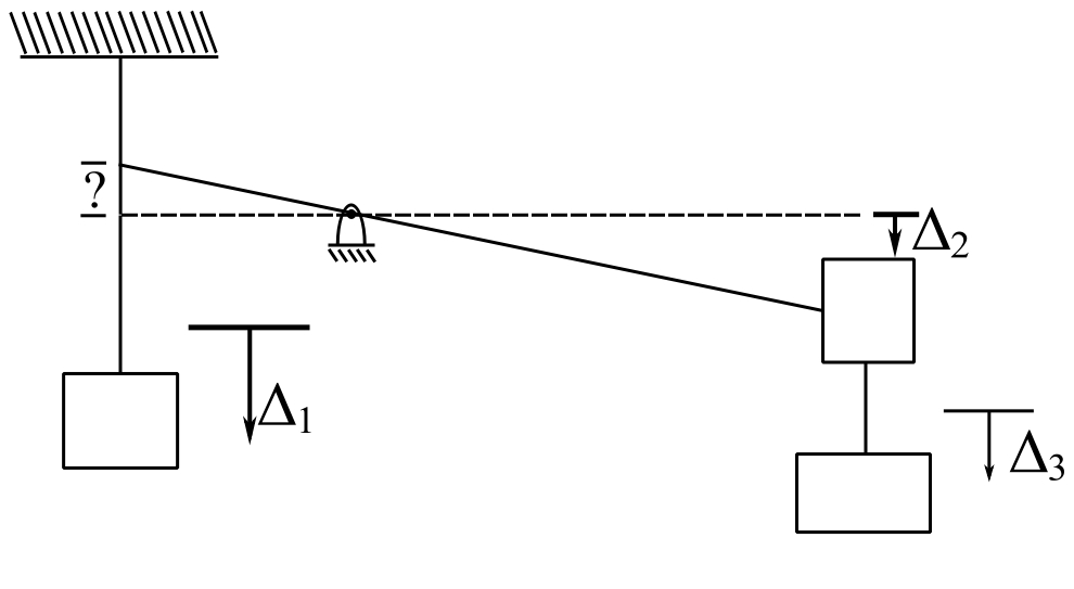
![\[F = 5mg\]](https://engcourses-uofa.ca/wp-content/ql-cache/quicklatex.com-b3278eb486b66413206e67043fbe4fde_l3.png "Rendered by QuickLaTeX.com")
![\[\Delta_1 = \frac{mg}k-5\frac{mg}k = -4\frac{mg}k\]](https://engcourses-uofa.ca/wp-content/ql-cache/quicklatex.com-ec445d9776c35b9284a8f8f1c9d370ac_l3.png "Rendered by QuickLaTeX.com")
![\[\Delta_2 = 15\frac{mg}k\]](https://engcourses-uofa.ca/wp-content/ql-cache/quicklatex.com-f9695ffba7d50e3e22fbbfbb78fba231_l3.png "Rendered by QuickLaTeX.com")
![\[\Delta_3 = 16\frac{mg}k\]](https://engcourses-uofa.ca/wp-content/ql-cache/quicklatex.com-eab2512dfdadf97b5b42295b8dad756a_l3.png "Rendered by QuickLaTeX.com")
Therefore choose 
![\[ m_{11} = m(4)(4) + m(-15)(-15) + m(-16)(-16) = 497m \]](https://engcourses-uofa.ca/wp-content/ql-cache/quicklatex.com-a50a1b1c604c5310126dc3a9dd99829c_l3.png "Rendered by QuickLaTeX.com")
![\[\begin{split} k_{11} &= k\begin{bmatrix} 4 && -15 && -16 \end{bmatrix} \begin{bmatrix} 1 && \frac{1}{3} && 0 \\ \frac{1}{3} && \frac{11}{9} && -1 \\ 0 && -1 && 1 \end{bmatrix} \begin{bmatrix} 4 \\ 15 \\ 16 \end{bmatrix} \\ &= 27k \end{split} \]](https://engcourses-uofa.ca/wp-content/ql-cache/quicklatex.com-d08511c867b69ebbcdcdfe9bdcf7bdd0_l3.png "Rendered by QuickLaTeX.com")
Therefore:
![\[ \begin{split} p_1 &= \sqrt{\frac{27}{497}}\sqrt{\frac{k}{m}} \\ &\leq 0.23308\sqrt{\frac{k}{m}} \end{split} \]](https://engcourses-uofa.ca/wp-content/ql-cache/quicklatex.com-def9e3e723c59c4e53894083e671052c_l3.png "Rendered by QuickLaTeX.com")
It is sometimes useful to consider these approximate solutions to finding the eigenvalues and eigenvectors. The UAMM gives upper bounds as do most techniques. We can get lower bounds as well.
Consider again the equations and motion.
![\[ \begin{bmatrix} m \end{bmatrix} \begin{Bmatrix} \Ddot{q} \end{Bmatrix} + \begin{bmatrix} k \end{bmatrix} \begin{Bmatrix} q \end{Bmatrix} = \begin{Bmatrix} 0 \end{Bmatrix} \]](https://engcourses-uofa.ca/wp-content/ql-cache/quicklatex.com-419147de0e76720d3a465a922f476883_l3.png "Rendered by QuickLaTeX.com")
To get to an eigenvalue problem we can do it in two ways.
- Premultiply by

![\[ \begin{split} \begin{Bmatrix} \begin{bmatrix} a \end{bmatrix} \begin{bmatrix} m \end{bmatrix} && - \frac{1}{p^2} \begin{bmatrix} I \end{bmatrix} \end{Bmatrix} \begin{Bmatrix} Q \end{Bmatrix} &= 0 \\ \begin{bmatrix} a \end{bmatrix} \begin{bmatrix} m \end{bmatrix} &:= \begin{bmatrix} D \end{bmatrix} -\text{dynamical matrix} \end{split} \]](https://engcourses-uofa.ca/wp-content/ql-cache/quicklatex.com-1f6b2ad65efe9450768d2af72f4b57d4_l3.png "Rendered by QuickLaTeX.com")
- Premultiply by

![\[ \begin{split} \begin{Bmatrix} \begin{bmatrix} m \end{bmatrix}^{-1} \begin{bmatrix} k \end{bmatrix} && - p^2 \begin{bmatrix} I \end{bmatrix} \end{Bmatrix} \begin{Bmatrix} Q \end{Bmatrix} &= 0 \\ \begin{bmatrix} m \end{bmatrix}^{-1} \begin{bmatrix} k \end{bmatrix} &:= \begin{bmatrix} \Delta \end{bmatrix} -\text{system matrix} \end{split} \]](https://engcourses-uofa.ca/wp-content/ql-cache/quicklatex.com-98a8268961a2adba8a21f99357d3de08_l3.png "Rendered by QuickLaTeX.com")
either gives the same eigenvalues and equivalent eigenvectors.
One can use these to find the eigenvalues/vectors through matrix iteration.
One clever idea that gives a lower bound is Dunkerleys formula. Consider the Dynamic Matrix formulation
![\[ \begin{Bmatrix} \begin{bmatrix} a \end{bmatrix} \begin{bmatrix} m \end{bmatrix} - \frac{1}{p^2}\begin{bmatrix} I \end{bmatrix} \end{Bmatrix} \begin{Bmatrix} Q \end{Bmatrix} = 0 \]](https://engcourses-uofa.ca/wp-content/ql-cache/quicklatex.com-511bbd1c4bfa104d2603b7b406d129bf_l3.png "Rendered by QuickLaTeX.com")
and expand the determinant of the coefficients
![\[ \begin{vmatrix} D_{11}-\frac{1}{p^2} && D_{12} && ... && D_{1n} \\ D_{21} && (D_{22}-\frac{1}{p^2} && ... && D_{2n} \\ \begin{matrix} . \\ . \\ . \end{matrix} && && && \\ D_{n1} && && && (D_{nn}-\frac{1}{p^2} \end{vmatrix} = 0 \]](https://engcourses-uofa.ca/wp-content/ql-cache/quicklatex.com-b0c4f7a54fdbb25858b6e39dae9602de_l3.png "Rendered by QuickLaTeX.com")
![\[ \biggr( \frac{1}{p^2} \biggr)^n - \big( D_{11} + D_{22} + D_{33} + ... + D_{nn} \big) \biggr( \frac{1}{p^2} \biggr)^{n-1} + ... = 0 \]](https://engcourses-uofa.ca/wp-content/ql-cache/quicklatex.com-e78c79e6c54e5f747cc047ddaf897fc3_l3.png "Rendered by QuickLaTeX.com")
Now consider that we have the roots of this polynomial  . This equation is equivalent to (factored)
![\[ \biggr( \frac{1}{p^2}-\frac{1}{p_1^2} \biggr) \biggr( \frac{1}{p^2}-\frac{1}{p_2^2} \biggr) \biggr( \frac{1}{p^2}-\frac{1}{p_3^2} \biggr) \biggr( \qquad \biggr) ... = 0 \]](https://engcourses-uofa.ca/wp-content/ql-cache/quicklatex.com-541587dd6c83aafdee633f80ebd63c19_l3.png "Rendered by QuickLaTeX.com")
and expand this to get
![\[ \biggr( \frac{1}{p^2} \biggr)^n - \biggr( \frac{1}{p_1^2} + \frac{1}{p_2^2} + \frac{1}{p_3^2} + ... + \frac{1}{p_n^2} \biggr) \biggr( \frac{1}{p^2} \biggr)^{n-1} + ... = 0 \]](https://engcourses-uofa.ca/wp-content/ql-cache/quicklatex.com-3b700449e0d03b2b4eda307bfc0c63ef_l3.png "Rendered by QuickLaTeX.com")
Now equate the coefficients
![\[ tr D = \biggr( \frac{1}{p_1^2} + \frac{1}{p_2^2} + ... + \frac{1}{p_n^2} \biggr) \]](https://engcourses-uofa.ca/wp-content/ql-cache/quicklatex.com-e90db29d39497579379821282cee93e4_l3.png "Rendered by QuickLaTeX.com")
However the largest term is the first one and often dominates
Therefore:
![\[ \begin{split} \frac{1}{p_1^2} &< tr D \\ p_1^2 &> \frac{1}{tr D} \end{split} \]](https://engcourses-uofa.ca/wp-content/ql-cache/quicklatex.com-2ec2cb5fbef31d06f86a032ab055b0fd_l3.png "Rendered by QuickLaTeX.com")
A special case occurs when the mass matrix is diagonal. Then tr D is
![\[ tr D = a_{11}m_1 + a_{22}m_2 + ... + a_{nn}m_{nn} \]](https://engcourses-uofa.ca/wp-content/ql-cache/quicklatex.com-61b2cc09566c28b6babeb9d10b12ea1e_l3.png "Rendered by QuickLaTeX.com")
and we need calculate only  to
to
In this case there is a physical interpretation of the expressions
![\[ \frac{1}{p_1^2} \leq a_{11}m_1 + a_{22}m_2 + a_{33}m_3... + a_{nn}m_{nn} \]](https://engcourses-uofa.ca/wp-content/ql-cache/quicklatex.com-d3eb23231a5a2475fe3d592e7dfe6833_l3.png "Rendered by QuickLaTeX.com")
namely that  is the natural frequency of the system with only
  as the mass (all other masses set to zero).
Therefore:
![\[ \frac{1}{p_1^2} \leq \frac{1}{p^2_{11}} + \frac{1}{p^2_{22}} + ... + \frac{1}{p^2_{nn}} \]](https://engcourses-uofa.ca/wp-content/ql-cache/quicklatex.com-07d99b304e9ca529f396751a2f06531b_l3.png "Rendered by QuickLaTeX.com")
This is also sometimes shown as Dunkerley’s formula.
Consider previous example
Calculate 
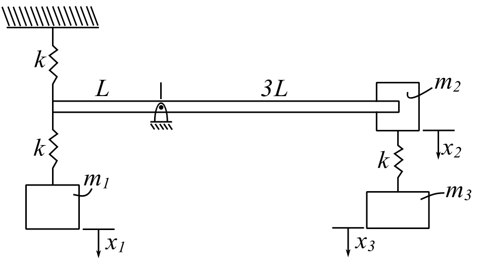
- Apply unit load to
![\[ \begin{split} \Delta_1 &= \frac{1}{k} + \frac{1}{k} = \frac{2}{k} = a_{11} \\ \Delta_2 &= -\frac{3}{k} = \Delta_3 \end{split} \]](https://engcourses-uofa.ca/wp-content/ql-cache/quicklatex.com-1b407dadd474be577bfef7566a1cb51d_l3.png "Rendered by QuickLaTeX.com")
Apply unit load to 
![\[ \begin{split} F(L) &= 1(3L) \\ F &= 3 \\ \hat{\Delta} &= \frac{3}{k} \\ a_{22} &= \frac{g}{k} \end{split} \]](https://engcourses-uofa.ca/wp-content/ql-cache/quicklatex.com-917d3d0e5066223b4ed1fb09a076a5a2_l3.png "Rendered by QuickLaTeX.com")
Apply unit load to 
![\[ \begin{split} \hat{\Delta} &= \frac{g}{k} \\ a_{33} &= \frac{9}{k} + \frac{1}{k} = \frac{10}{k} \end{split} \]](https://engcourses-uofa.ca/wp-content/ql-cache/quicklatex.com-81486d47bf1945c35e098236fa092987_l3.png "Rendered by QuickLaTeX.com")
Therefore:
![\[ \begin{split} \frac{1}{p_1^2} &< m\left(\frac{2}{k}\right) + m\left(\frac{9}{k}\right) + m\left(\frac{10}{k}\right) = \frac{21m}{k} \\ p_1 &> \sqrt{\frac{1}{21}}\sqrt{\frac{k}{m}} = \underline{0.2182\sqrt{\frac{k}{m}}} \end{split} \]](https://engcourses-uofa.ca/wp-content/ql-cache/quicklatex.com-a07c60b169ff5e0d0665a510ef283357_l3.png "Rendered by QuickLaTeX.com")
Consider an example of a continuous system
![\[ \begin{split} \phi_1 &= x^2 \\ \phi^{''}_1 &= 2 \\ \phi_2 &= x^3 \\ \phi^{''}_2 &= 6x \end{split} \]](https://engcourses-uofa.ca/wp-content/ql-cache/quicklatex.com-4d610558e7d842ceb095c938918682ae_l3.png "Rendered by QuickLaTeX.com")
![\[ \begin{split} m_{ij} &= \int_m \phi_i\phi_j dm \\ &= \int_0^L \phi_i\phi_J mdx \qquad \text{where } m= \text{ mass/length} \end{split} \]](https://engcourses-uofa.ca/wp-content/ql-cache/quicklatex.com-d35f952f4408a01fce3ae0799fcba245_l3.png "Rendered by QuickLaTeX.com")
![\[ \begin{split} m_{11} &= m\int_0^L x^4 dx = \frac{mL^5}{5} \\ m_{12} &= m\int_0^L x^5dx = \frac{mL^6}{6} = m_{21} \\ m_{22} &= \frac{mL^7}{7} \end{split} \]](https://engcourses-uofa.ca/wp-content/ql-cache/quicklatex.com-caaa4871e1b3f017c277c5f519669b3b_l3.png "Rendered by QuickLaTeX.com")
![\[ \begin{split} k_{ij} &= \int EI\phi_i''\phi_j'' dx \\ k_{11} &= EI \int_0^L 4 dx\\ &= EI(4L) \\ k_{12} &= EI\int_0^L 12x dx \\ &= 6EIL^2 \\ k_{22} &= 12L^3EI \end{split} \]](https://engcourses-uofa.ca/wp-content/ql-cache/quicklatex.com-eb1d6e618aedf8dfe2cf5b38bbc8b4fb_l3.png "Rendered by QuickLaTeX.com")
![\[ mL^5 \begin{bmatrix} 1/5 && L/6 \\ L/6 && L^2/7 \end{bmatrix} \begin{Bmatrix} \Ddot{q}_1 \\ \Ddot{q}_2 \end{Bmatrix} + EIL \begin{bmatrix} 4 && 6L \\ 6L && 12L^2 \end{bmatrix} \begin{Bmatrix} q_1 \\ q_2 \end{Bmatrix} = \begin{Bmatrix} 0 \\ 0 \end{Bmatrix} \]](https://engcourses-uofa.ca/wp-content/ql-cache/quicklatex.com-f65be4d486b656d6ad31d27b0057b51b_l3.png "Rendered by QuickLaTeX.com")
Therefore the eigenvalue problem is
![\[ \begin{bmatrix} 4 - \frac{\lambda}{5} && 6L - \frac{\lambda L}{6} \\ 6L - \frac{\lambda L}{6} && 12L^2 - L^2 \frac{\lambda}{7} \end{bmatrix} \begin{Bmatrix} Q_1 \\ Q_2 \end{Bmatrix} = \begin{Bmatrix} 0 \\ 0 \end{Bmatrix} \]](https://engcourses-uofa.ca/wp-content/ql-cache/quicklatex.com-243ef28d882edc7a8b607a0592695310_l3.png "Rendered by QuickLaTeX.com")
![\[ \begin{split} (4-\frac{\lambda}{5})L^2(12-\frac{\lambda}{7}) - L^2(6-\frac{\lambda}{6})^2 &= 0 \\ 48 - \frac{12}{5}\lambda - \frac{4}{7}\lambda + \frac{\lambda^2}{35} - (36-2\lambda + \frac{\lambda^2}{36}) &= 0 \\ 12 - \frac{(84+20-70)}{35}\lambda + \lambda^2(\frac{1}{35}-\frac{1}{36}) &= 0 \\ 12(35)(36) - (34)(36)\lambda + \lambda^2 &= 0 \end{split} \]](https://engcourses-uofa.ca/wp-content/ql-cache/quicklatex.com-a281ead069b6d1bf2aaafb5d96ab2fac_l3.png "Rendered by QuickLaTeX.com")
![\[ \lambda^2 - (34)(36)\lambda - 12(35)(36) \]](https://engcourses-uofa.ca/wp-content/ql-cache/quicklatex.com-5a95944e0a9f63c1ed416a1099810172_l3.png "Rendered by QuickLaTeX.com")
![\[ \begin{split} \lambda &= (34)(18) \pm \sqrt{(34)^2(18)^2 - 12(35)(36)} \\ &= 612 \pm \sqrt{359424} \\ &= 612 \pm 599.5 \\ &= 12.48, 1211.5 \end{split} \]](https://engcourses-uofa.ca/wp-content/ql-cache/quicklatex.com-88b8ed4dba4238b51488a3d5479e0c11_l3.png "Rendered by QuickLaTeX.com")
Therefore
![\[ \begin{split} p_1^2 &= \sqrt{12.48} \sqrt{\frac{EI}{mL^4}} \\ &= 3.53\sqrt{\frac{EI}{mL^4}} \\ p_2^2 &= 34.8 \sqrt{\frac{EI}{mL^4}} \end{split} \]](https://engcourses-uofa.ca/wp-content/ql-cache/quicklatex.com-8a4eb45e7dde7c276a0c14e558e1a9a8_l3.png "Rendered by QuickLaTeX.com")
![\[ (4-\frac{\lambda}{5})q_1 + (6-\frac{\lambda}{6})Lq_2 = 0 \]](https://engcourses-uofa.ca/wp-content/ql-cache/quicklatex.com-ce840344cba7323a6aab87fb7957b7b8_l3.png "Rendered by QuickLaTeX.com")
![\[ \begin{split} \frac{Lq_2}{q_1} &= \frac{-(4-\frac{\lambda}{5})}{(6-\frac{\lambda}{6})} \\ &= \frac{-(4-\frac{12.48}{5})}{6-\frac{12.48}{6}} \\ &= -0.384 \end{split} \]](https://engcourses-uofa.ca/wp-content/ql-cache/quicklatex.com-3d1ceae71053f0dd4e3aa4e46a6fdf39_l3.png "Rendered by QuickLaTeX.com")
The mode shape is
![\[ \phi = x^2 - 0.384x^3 \]](https://engcourses-uofa.ca/wp-content/ql-cache/quicklatex.com-00510da03aab2a6c6cb40e33af09c85e_l3.png "Rendered by QuickLaTeX.com")
What if we apply some dynamic loading to the structure? Then we must calculate the generalized forces for our model. Consider a virtual displacement
![\[ \delta_y = \sum_{i=1}^n \phi_i(x)\delta q_i \]](https://engcourses-uofa.ca/wp-content/ql-cache/quicklatex.com-9e88ab383bec5c9cd3fb6bc109be635d_l3.png "Rendered by QuickLaTeX.com")
then
![\[ \begin{split} \delta W &= \sum_{j=1}^m F_j \biggr( \sum_{i=1}^n \phi_i (x_j) \delta_{q_i} \biggr) \\ &= \sum_{i=1}^n \delta_{q_i} \biggr( \sum_{j=1}^m F_j \phi_i (x_j) \biggr) \\ &= \sum_{i=1}^n Q_i \delta q_i \end{split} \]](https://engcourses-uofa.ca/wp-content/ql-cache/quicklatex.com-a1e614f1d6c9f34853cc1eef60b3cafa_l3.png "Rendered by QuickLaTeX.com")
Therefore
![\[ Q_i = \sum_{j=1}^m F_j \phi_i (x_j) \]](https://engcourses-uofa.ca/wp-content/ql-cache/quicklatex.com-de5a9956335afd723db8ef05403e3732_l3.png "Rendered by QuickLaTeX.com")
Consider the previous example
![\[ \begin{split} Q_1 &= F(t) \phi_1 (L) = F(t) L^2 \\ Q_2 &= F(t) \phi_2 (L) = F(t) L^3\end{split} \]](https://engcourses-uofa.ca/wp-content/ql-cache/quicklatex.com-8d7e0b6b7cc9ec3d921342f248d7f10d_l3.png "Rendered by QuickLaTeX.com")
![\[ \begin{bmatrix} m \end{bmatrix} \begin{Bmatrix} \Ddot{q} \end{Bmatrix} + \begin{bmatrix} k \end{bmatrix} \begin{Bmatrix} q \end{Bmatrix} = F(t) \begin{Bmatrix} L^2 \\ L^3 \end{Bmatrix} \]](https://engcourses-uofa.ca/wp-content/ql-cache/quicklatex.com-9190faa724a7dd0c92bf37e79276f3c7_l3.png "Rendered by QuickLaTeX.com")
Whirling of Rotating Shafts
Rotating shafts tend to bow out at certain speeds and whirl in a complicated manner. Whirling is defined as the rotation of the bent shaft and the line of centers of the bearing. This phenomenon results from various causes as mass unbalance, hysteresis damping, gyroscopic effects, fluid friction, etc. This whirling can take place in the same or opposite direction as that of the rotation of the shaft. The whirling speed may or may not be equal to the rotation speed.
Let us assume a simple system
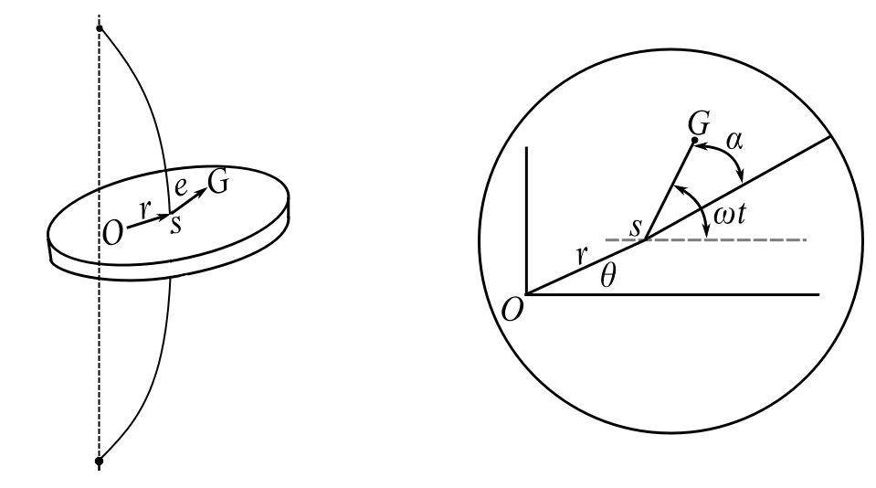
Note:  is the center of the disc,
  is the center of gravity, and
  is an eccentricity.
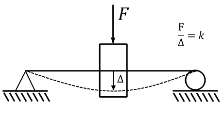
is the stiffness of the system to lateral deflection.
We will assume the shaft to be rotating at an instant angular velocity  and OS to be whirling at angular speed
![\[ \underline{v}_G = \underline{v}_s + v_{G/s} \]](https://engcourses-uofa.ca/wp-content/ql-cache/quicklatex.com-3e6b630900430fe53a670c4b7028b547_l3.png "Rendered by QuickLaTeX.com")
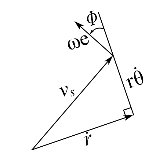
Where 
![\[ \begin{split} v_r^G &= \dot{r} - e\omega\sin(\omega t - \theta) \\ v_\theta^G &= r\dot{\theta} + \omega e\cos(\omega t - \theta) \end{split} \]](https://engcourses-uofa.ca/wp-content/ql-cache/quicklatex.com-3c854a8d50698b156dd9eb64813cb1bb_l3.png "Rendered by QuickLaTeX.com")
Therefore:
![\[ \begin{split} \Big( v^G \big)^2 &= \Big[ \dot{r} - e\omega \sin(\omega t - \theta)\Big]^2 + \Big[ r\dot{\theta} + e\omega \cos(\omega t - \theta)\Big]^2 \\ &= (\dot{r})^2 - 2\dot{r}e\omega\sin(\omega t - \theta) + (r\dot{\theta})^2 + 2r\dot{\theta}e\omega\cos(\omega t - \theta) + e^2\omega^2 \\ (v_G)^2 &= (\dot{r})^2 + (r\dot{\theta})^2 + e^2\omega^2 - 2\dot{r}e\omega\sin(\omega t -\theta) + 2r\dot{\theta}e\omega\cos(\omega t -\theta) \end{split} \]](https://engcourses-uofa.ca/wp-content/ql-cache/quicklatex.com-0089dd63585e6b26f51b365e8245afea_l3.png "Rendered by QuickLaTeX.com")
Therefore:
![\[ \begin{split} T &= \frac{1}{2} J_G \omega^2 + \frac{1}{2}mv^2_G \\ V &= \frac{1}{2}kr^2 \\ L &= T - V \end{split} \]](https://engcourses-uofa.ca/wp-content/ql-cache/quicklatex.com-4b2483a3ac4f9d02fac2cb9a1b6ab4d5_l3.png "Rendered by QuickLaTeX.com")
Therefore:
![\[ \begin{split} \frac{d}{dt}\Big(\frac{\partial L}{\partial\dot{r}}\Big) - \frac{\partial L}{\partial r} &= Q_r \\ \frac{d}{dt}\Big(\frac{\partial L}{\partial\dot{\theta}}\Big) - \frac{\partial L}{\partial\theta} &= Q_\theta \end{split} \]](https://engcourses-uofa.ca/wp-content/ql-cache/quicklatex.com-e4ad4a18364a95e6f4de1a875bb119ad_l3.png "Rendered by QuickLaTeX.com")
![\[ \begin{split} \frac{\partial (V_G)^2}{\partial \dot{\theta}} &= 2r^2\dot{\theta} + 2re\omega\cos(\omega t - \theta) \\ \frac{\partial (V_G)^2}{\partial \dot{r}} &= 2\dot{r} - 2e\omega\sin(\omega t - \theta) \\ \frac{\partial (V_G)^2}{\partial \theta} &= 2\dot{r}e\omega\cos(\omega t -\theta) + 2r\theta e\omega\sin(\omega t - \theta) \\ \frac{\partial (V_G)^2}{\partial r} &= 2r(\dot{\theta})^2 + 2\dot{\theta}e\omega\cos(\omega t - \theta) \end{split} \]](https://engcourses-uofa.ca/wp-content/ql-cache/quicklatex.com-199350d6ac27c0327970071edd05eefc_l3.png "Rendered by QuickLaTeX.com")
Therefore:
![\[ \begin{split} \frac{md}{2dt}\big[2\dot{r}-2e\omega\sin(\omega t-\theta)\big] - \frac{m}{2}\big[2r(\dot{\theta}^2)+2\dot{\theta} e\omega\cos(\omega t -\theta) + kr &= -c\dot{r} \\ m\Ddot{r} - me\omega\cos(\omega t - \theta)(\omega - \dot{\theta}) - mr(\dot{\theta})^2 - m\dot{\theta}e\omega\cos(\omega t - \theta) + kr &= 0 \\ m\Ddot{r} - mr(\dot{\theta})^2 - me\omega^2\cos(\omega t -\theta) + kr &= -c\dot{r} \end{split} \]](https://engcourses-uofa.ca/wp-content/ql-cache/quicklatex.com-34edd448effa579679f22e435d04515f_l3.png "Rendered by QuickLaTeX.com")
Therefore:
![\[ \Ddot{r} + \frac{k}{m}r + \frac{c}{m}\dot{r}-r(\dot{\theta})^2 = e\omega^2\cos(\omega t - \theta) \]](https://engcourses-uofa.ca/wp-content/ql-cache/quicklatex.com-0ced5df91c70aff5b2015eb9e6e10ee6_l3.png "Rendered by QuickLaTeX.com")
![\[ \frac{d}{dt}\Big(\frac{\partial L}{\partial \dot{\theta}}\Big) - \frac{\partial L}{\partial \theta} \]](https://engcourses-uofa.ca/wp-content/ql-cache/quicklatex.com-cb7640142b546742b9e8995abb6b5c4d_l3.png "Rendered by QuickLaTeX.com")
![\[ \begin{split} &\frac{m}{2}\frac{d}{dt}\big(2r^2\dot{\theta} + 2re\omega\cos(\omega t -\theta)\big) - \frac{m}{2}\big[2\dot{r}e\omega\cos(\omega t - \theta) + 2r\dot{\theta}e\omega\sin(\omega t -\omega)\big] \\ &= m\big[ 2r\dot{r}\dot{\theta} + r^2\Ddot{\theta} + \dot{r}e\omega\cos(\omega t -\theta) - re\omega(\omega - \dot{\theta})\sin(\omega t - \theta)\big] \\ &- m\big[\dot{r}e\omega\cos(\omega t - \theta) + r\dot{\theta}e\omega\sin(\omega t - \theta)\big] \end{split} \]](https://engcourses-uofa.ca/wp-content/ql-cache/quicklatex.com-5cb85c2ea2a345bcd8b8a59e24e83706_l3.png "Rendered by QuickLaTeX.com")
Therefore:
![\[ mr\Ddot{\theta} + 2m\dot{r}\dot{\theta} - me\omega^2\sin(\omega t - \theta) = -cr\Ddot{\theta} \]](https://engcourses-uofa.ca/wp-content/ql-cache/quicklatex.com-8a669e581e39e2fa9cb4cd40ead8989a_l3.png "Rendered by QuickLaTeX.com")
Therefore:
![\[ r\Ddot{\theta} + \frac{c}{m}r\dot{\theta} + 2\dot{r}\dot{\theta} = e\omega^2\sin(\omega t - \theta) \]](https://engcourses-uofa.ca/wp-content/ql-cache/quicklatex.com-5381f85dae4800bd272270e8b476752e_l3.png "Rendered by QuickLaTeX.com")
These are nonlinear equations and there are more than one solution.
Consider the simplest case of synchronous whirl i.e. try
![\[ \begin{split} \dot{\theta} &= \omega \qquad \theta = \omega t - \phi \\ \Ddot{\theta} &= 0 \qquad \Ddot{r} = \dot{r} = 0 \end{split} \]](https://engcourses-uofa.ca/wp-content/ql-cache/quicklatex.com-68d382cb9128f9c415aad7c89b6d5102_l3.png "Rendered by QuickLaTeX.com")
Therefore:
![\[ \begin{split} \frac{k}{m}r - r\omega^2 &= e\omega^2\cos\phi \\ \frac{c}{m}r\omega &= e\omega^2\sin\phi \\ r\Big(\frac{k}{m} - \omega^2\Big) &= e\omega^2\cos\phi \end{split} \]](https://engcourses-uofa.ca/wp-content/ql-cache/quicklatex.com-7dd13c4c238366474b90d03ca2c11fe4_l3.png "Rendered by QuickLaTeX.com")
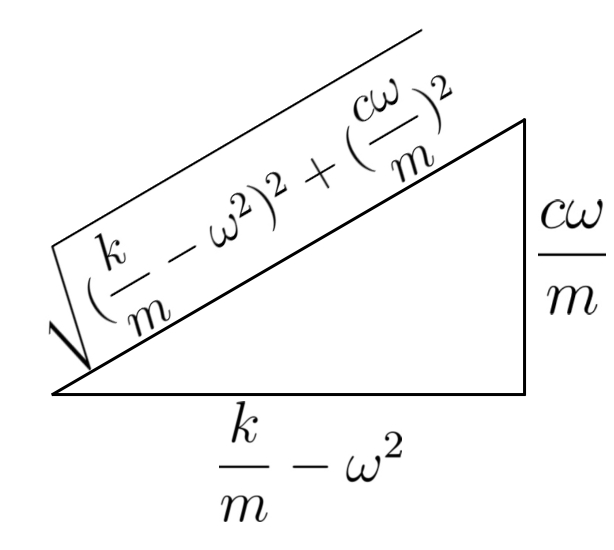
![\[ \begin{split} \tan\phi &= \frac{\frac{c}{m}r\omega}{r\big(\frac{k}{m}-\omega^2\big)} \\ p &= \frac{k}{m} \\ \zeta &= 2mp \end{split} \]](https://engcourses-uofa.ca/wp-content/ql-cache/quicklatex.com-cbecce8cca331d353ea9336503ed08a4_l3.png "Rendered by QuickLaTeX.com")
![\[ \begin{split} r &= \frac{e\omega^2}{\big(\frac{k}{m}-\omega^2\big)}\cos\phi \\ &= \frac{e\omega^2}{\big(\frac{k}{m}-\omega^2\big)} \frac{\big(\frac{k}{m}-\omega^2\big)}{\sqrt{\big(\frac{k}{m}-\omega^2\big)^2+\big(\frac{c}{m}\omega\big)^2}} \end{split} \]](https://engcourses-uofa.ca/wp-content/ql-cache/quicklatex.com-363db2d85ef22589760888fdb0ab3075_l3.png "Rendered by QuickLaTeX.com")
![\[ r = \frac{e\big(\frac{\omega}{p}\big)^2}{\sqrt{\big(1-\big(\frac{\omega}{p}\big)^2\big)^2 + \big( 2\zeta\frac{\omega}{p}\big)^2 }} \]](https://engcourses-uofa.ca/wp-content/ql-cache/quicklatex.com-ede14a1318c2d9cc1b0635fef92f0e18_l3.png "Rendered by QuickLaTeX.com")
This looks exactly the same as rotating inbalance excitation
Therefore the
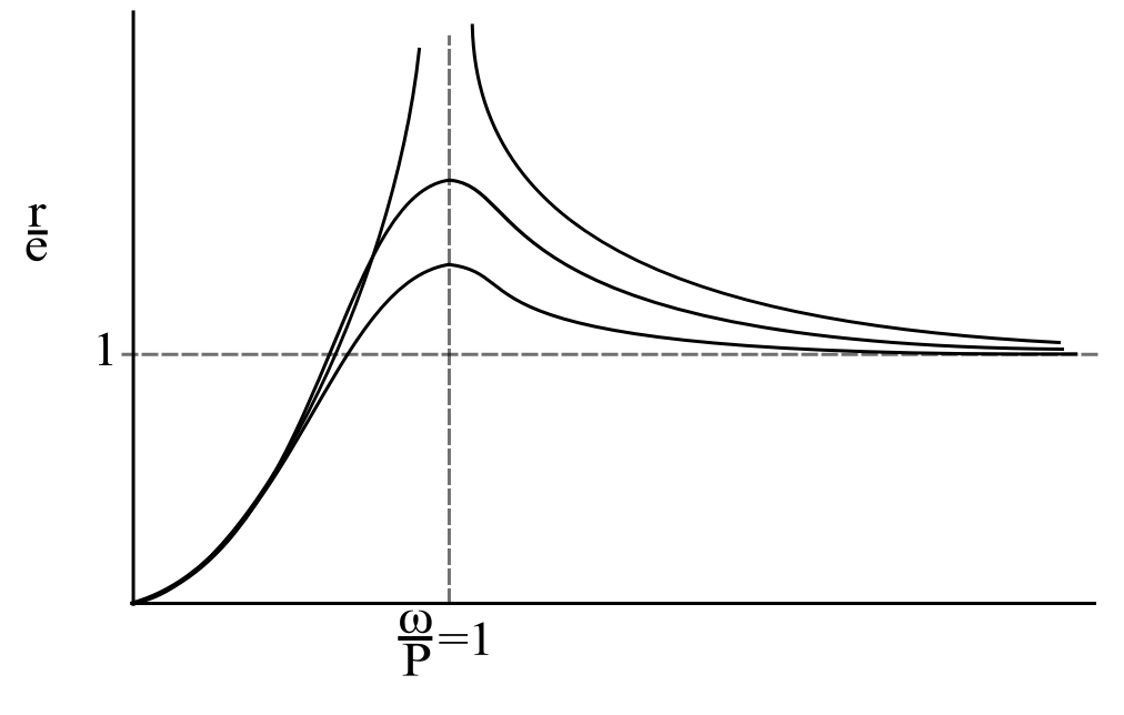
So that synchronous whirl occurs when 
Self Excited Vibrations
Almost all of the vibrations considered so far were either free or forced vibrations. A fundamentally different class are the so-called self-excited vibrations.
“In a self-excited vibration the alternating force that sustains the motion is created or controlled by the motion itself ; when the motion stops the alternating force disappears”
In a forced vibration the sustaining alternating force exists independently of the motion and persists even when the vibratory motion is stopped.
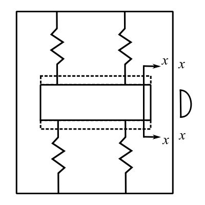
Engineered art
- Use vibration phenomena for the display of classic ideas that ask the question “Why does that occur”
- Search kinetic art
- Naum Gabo Stationary Wave (1919)
Spinning Pendulum
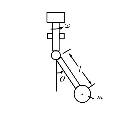
Consider the stability of the SHM of the simple pendulum that is rotating with angular velocity . The total velocity of mass is:
![\[\nu^2 = (\ell\dot\theta)^2+(\ell\theta\omega)^2\]](https://engcourses-uofa.ca/wp-content/ql-cache/quicklatex.com-39699cc57acb5842afa3705c09245fe0_l3.png "Rendered by QuickLaTeX.com")
![\[T = \frac{1}{2}m\ell^2[\dot\theta^2+\theta^2\omega^2]\]](https://engcourses-uofa.ca/wp-content/ql-cache/quicklatex.com-60bce91174eb3fbaa7948782da9ee176_l3.png "Rendered by QuickLaTeX.com")
![\[\begin{split}V &= mg\ell[1-\cos\theta ] \\&=\frac{1}{2}mg\ell\theta^2\end{split}\]](https://engcourses-uofa.ca/wp-content/ql-cache/quicklatex.com-e886b69dd84c6f5d9537198a9bee0513_l3.png "Rendered by QuickLaTeX.com")
![\[\frac{d}{dt}\bigg(\frac{\partial L}{\partial\dot\theta}\bigg)-\frac{\partial L}{\partial \theta} = 0\]](https://engcourses-uofa.ca/wp-content/ql-cache/quicklatex.com-c01d13295d6d233c0cf011e19e71bc80_l3.png "Rendered by QuickLaTeX.com")
![\[m\ell^2\ddot\theta- m\ell^2\theta\omega^2+mg\ell\theta=0\]](https://engcourses-uofa.ca/wp-content/ql-cache/quicklatex.com-45623fecae7ae28b49e58a06a7d146a3_l3.png "Rendered by QuickLaTeX.com")
![\[\ddot\theta+\bigg(\frac{g}{\ell}-\omega^2\bigg)\theta = 0\]](https://engcourses-uofa.ca/wp-content/ql-cache/quicklatex.com-10b59d5e0afce7be55319f0a84baff7e_l3.png "Rendered by QuickLaTeX.com")
![\[p^2 = \frac{g}{\ell} - \omega^2\]](https://engcourses-uofa.ca/wp-content/ql-cache/quicklatex.com-bbd017b0ed96eda168bac020f4a718c5_l3.png "Rendered by QuickLaTeX.com")
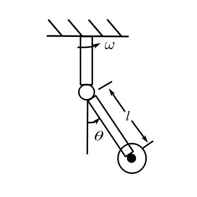
The frequency of oscillation of the pendulum is:
![\[ f_p = \frac{1}{2\pi}\sqrt{\frac{q}{\ell}-\omega^2}\]](https://engcourses-uofa.ca/wp-content/ql-cache/quicklatex.com-e41d3b3927bc8d83d60bc9ecd2daf1b5_l3.png "Rendered by QuickLaTeX.com")
Therefore the pendulum will oscillate ( ) until
  at which point the pendulum will simply fly horizontally and never cross the
  .
.
To see the frequencies try a length of pendulum of  inches.
When  :
:
![\[\begin{split} f_p &=\frac{1}{2\pi}\sqrt{\frac{386}{8}} \\&=\underline{\underline{1.1}}\text{ Hz (66 RPM)}\end{split}\]](https://engcourses-uofa.ca/wp-content/ql-cache/quicklatex.com-96b6835da1e64254dbd75c0103d8880b_l3.png "Rendered by QuickLaTeX.com")
When  RPM:
RPM:
![\[\begin{split} f_p &=\frac{1}{2\pi}\sqrt{\frac{386}{8}- \bigg(\frac{2\pi \cdot30}{60}\bigg)^2} \\& = \underline{\underline{0.99}}\text{ Hz}\end{split}\]](https://engcourses-uofa.ca/wp-content/ql-cache/quicklatex.com-9e9e106e05886720aea8ec1cd8cd0add_l3.png "Rendered by QuickLaTeX.com")
When  RPM:
RPM:
![\[\begin{split} f_p &=\frac{1}{2\pi}\sqrt{\frac{386}{8}- \bigg(\frac{2\pi \cdot40}{60}\bigg)^2} \\& = \underline{\underline{0.88}}\text{ Hz}\end{split}\]](https://engcourses-uofa.ca/wp-content/ql-cache/quicklatex.com-c8ea39565df096ece926cbda73cb7f66_l3.png "Rendered by QuickLaTeX.com")
When  RPM:
RPM:
![\[\begin{split} f_p &=\frac{1}{2\pi}\sqrt{\frac{386}{8}- \bigg(\frac{2\pi \cdot50}{60}\bigg)^2} \\& = \underline{\underline{0.73}}\text{ Hz}\end{split}\]](https://engcourses-uofa.ca/wp-content/ql-cache/quicklatex.com-10808d47f6b82ccd09d562b371442678_l3.png "Rendered by QuickLaTeX.com")
When  RPM:
RPM:
![\[\begin{split} f_p &=\frac{1}{2\pi}\sqrt{\frac{386}{8}- \bigg(\frac{2\pi \cdot60}{60}\bigg)^2} \\& = \underline{\underline{0.47}}\text{ Hz}\end{split}\]](https://engcourses-uofa.ca/wp-content/ql-cache/quicklatex.com-ecdf00171eeb2a87ffd35344bbaba2eb_l3.png "Rendered by QuickLaTeX.com")
Friction Testing (Kinetic)
![\[ w=mg\]](https://engcourses-uofa.ca/wp-content/ql-cache/quicklatex.com-e70631473a9dfbcd3f2e214224454966_l3.png "Rendered by QuickLaTeX.com")
![\[ \begin{split} +\uparrow\sum F_y &= R_1 + R_2 - mg = 0 \qquad \textcircled{1} \\ +\rightarrow\sum F_x &= \mu(R_1-R_2) = m\Ddot{x} \qquad \textcircled{2} \\ +\circlearrowleft\sum M_G &= 0 = \mu(R_1-R_2)h + R_2(a-x) - R_1(a+x) \qquad \textcircled{3} \end{split} \]](https://engcourses-uofa.ca/wp-content/ql-cache/quicklatex.com-37c8bb250607bfd7d9824837e7ae0c32_l3.png "Rendered by QuickLaTeX.com")
Find the natural frequency in terms of 
From
![\[ R_1 + R_2 = mg \qquad \textcircled{4} \]](https://engcourses-uofa.ca/wp-content/ql-cache/quicklatex.com-ccddcbc91325132da83ebd7b196e48d9_l3.png "Rendered by QuickLaTeX.com")
From
![\[ (R_1 - R_2)\mu h + (R_2 - R_1)a - (R_1 + R_2)x = 0 \]](https://engcourses-uofa.ca/wp-content/ql-cache/quicklatex.com-939c9c5fd9a30d3620a69fcfe82ce7c9_l3.png "Rendered by QuickLaTeX.com")
Using 
![\[ (R_1 - R_2)\mu h + (R_2 - R_1)a - mgx = 0 \]](https://engcourses-uofa.ca/wp-content/ql-cache/quicklatex.com-8c8081ed544ded8758375aec87eae704_l3.png "Rendered by QuickLaTeX.com")
Therefore:
![\[ \begin{split} (R_1 - R_2)(\mu h - a) &= mgx \\ (R_1 - R_2) &= \frac{mgx}{(\mu h - a)} \end{split} \]](https://engcourses-uofa.ca/wp-content/ql-cache/quicklatex.com-8dd455163163d770e8230ccd05be162c_l3.png "Rendered by QuickLaTeX.com")
From
![\[ \frac{\mu mgx}{(\mu h - a)} = m\Ddot{x} \]](https://engcourses-uofa.ca/wp-content/ql-cache/quicklatex.com-62d960f3266f27c27819a7532eaeb676_l3.png "Rendered by QuickLaTeX.com")
![\[ \Ddot{x} + \frac{\mu g}{a - \mu h}x = 0 \]](https://engcourses-uofa.ca/wp-content/ql-cache/quicklatex.com-ae8538e007c7c49c89c1b73a19cf10dc_l3.png "Rendered by QuickLaTeX.com")
Therefore:
![\[ p^2 = \sqrt{\frac{\mu g}{a - \mu h}} \]](https://engcourses-uofa.ca/wp-content/ql-cache/quicklatex.com-5f4e2bc7d8e49204f33dac506a6aaca4_l3.png "Rendered by QuickLaTeX.com")
Therefore, frequency of oscillation is
![\[ f = \frac{1}{2\pi}\sqrt{\frac{\mu g}{a - \mu h}} \]](https://engcourses-uofa.ca/wp-content/ql-cache/quicklatex.com-854f060104554aa266d0b2edd84fd4c1_l3.png "Rendered by QuickLaTeX.com")
“Friction keeps the world in harmonious motion”
![\[ a = 4" \qquad \mu = 0.5 \qquad h = 1" \]](https://engcourses-uofa.ca/wp-content/ql-cache/quicklatex.com-f8cf81d2f721790f80e06e11f97b86f3_l3.png "Rendered by QuickLaTeX.com")
![\[ f = \frac{1}{2\pi} \sqrt{\frac{(0.5)386}{4 - (0.5)}} = \underline{1.2 \text{ Hz}} \]](https://engcourses-uofa.ca/wp-content/ql-cache/quicklatex.com-084f2dc3358db7f4176c869b4e0d4938_l3.png "Rendered by QuickLaTeX.com")
![\[ a = 4 \qquad \mu = 0.1 \qquad h = 1" \]](https://engcourses-uofa.ca/wp-content/ql-cache/quicklatex.com-e3879df168d9139540597d4bf258b551_l3.png "Rendered by QuickLaTeX.com")
![\[ f = \frac{1}{2\pi} \sqrt{\frac{(0.1)386}{4 - (0.1)}} = \underline{0.5 \text{ Hz}} \]](https://engcourses-uofa.ca/wp-content/ql-cache/quicklatex.com-888c3cb0c6a0065d4ce4e7da88c6339e_l3.png "Rendered by QuickLaTeX.com")
![\[f = \frac{1}{2\pi}\sqrt{\frac{\mu g}{\alpha - \mu h}} \]](https://engcourses-uofa.ca/wp-content/ql-cache/quicklatex.com-3252ed07088d8b30723d1f036d0f2aaf_l3.png "Rendered by QuickLaTeX.com")
Let  ,
,  and
and  :
:
![\[ \begin{split} f &= \frac{1}{2\pi}\sqrt{\frac{(0.1)(386)}{3 - (0.1)(0.5)}} \\&= 0.576 \text{ Hz} \end{split} \]](https://engcourses-uofa.ca/wp-content/ql-cache/quicklatex.com-c781ee23f10aece5749aff8022660937_l3.png "Rendered by QuickLaTeX.com")
If  :
:
![\[ \begin{split} f &= \frac{1}{2\pi}\sqrt{\frac{(0.2)(386)}{3 - (0.2)(0.5)}} \\&= 0.821 \text{ Hz} \end{split} \]](https://engcourses-uofa.ca/wp-content/ql-cache/quicklatex.com-42e3a955c4ff26002cac05e8b84bf127_l3.png "Rendered by QuickLaTeX.com")
If  (TEFLON/STEEL):
![\[ \begin{split} f &= \frac{1}{2\pi}\sqrt{\frac{(0.04)(386)}{3 - (0.04)(0.5)}} \\&= 0.361 \text{ Hz} \end{split} \]](https://engcourses-uofa.ca/wp-content/ql-cache/quicklatex.com-0ad4f490feba296b37ff9b623179d4bb_l3.png "Rendered by QuickLaTeX.com")
If  :
:
![\[ \begin{split} f &= \frac{1}{2\pi}\sqrt{\frac{(0.3)(386)}{3 - (0.3)(0.5)}} \\&= 1.01 \text{ Hz} \end{split} \]](https://engcourses-uofa.ca/wp-content/ql-cache/quicklatex.com-a7944dc94c8f303f67ab1837d0f7d048_l3.png "Rendered by QuickLaTeX.com")
If  :
:
![\[ \begin{split} f &= \frac{1}{2\pi}\sqrt{\frac{(0.4)(386)}{3 - (0.4)(0.5)}} \\&= 1.18 \text{ Hz} \end{split} \]](https://engcourses-uofa.ca/wp-content/ql-cache/quicklatex.com-bc7285979d3ae8759728d19994599d35_l3.png "Rendered by QuickLaTeX.com")
If  :
:
![\[ \begin{split} f &= \frac{1}{2\pi}\sqrt{\frac{(0.5)(386)}{3 - (0.5)(0.5)}} \\&= 1.33 \text{ Hz} \end{split} \]](https://engcourses-uofa.ca/wp-content/ql-cache/quicklatex.com-ff3759c29ba8d1eb864f87932eb814f3_l3.png "Rendered by QuickLaTeX.com")
If  :
:
![\[ \begin{split} f &= \frac{1}{2\pi}\sqrt{\frac{(0.6)(386)}{3 - (0.6)(0.5)}} \\&= 1.47 \text{ Hz} \end{split} \]](https://engcourses-uofa.ca/wp-content/ql-cache/quicklatex.com-04b293a856355463f1e353e2f77c6a6f_l3.png "Rendered by QuickLaTeX.com")
If  :
:
![\[ \begin{split} f &= \frac{1}{2\pi}\sqrt{\frac{(0.7)(386)}{3 - (0.7)(0.5)}} \\&= 1.61 \text{ Hz} \end{split} \]](https://engcourses-uofa.ca/wp-content/ql-cache/quicklatex.com-7be4efed8cd3c5d30738fb75a16e78b5_l3.png "Rendered by QuickLaTeX.com")
If  :
:
![\[ \begin{split} f &= \frac{1}{2\pi}\sqrt{\frac{(0.8)(386)}{3 - (0.8)(0.5)}} \\&= 1.73 \text{ Hz} \end{split} \]](https://engcourses-uofa.ca/wp-content/ql-cache/quicklatex.com-500583b58b6aa2a16e292767746df7b5_l3.png "Rendered by QuickLaTeX.com")
If  :
:
![\[ \begin{split} f &= \frac{1}{2\pi}\sqrt{\frac{(0.9)(386)}{3 - (0.9)(0.5)}} \\&= 1.86 \text{ Hz} \end{split} \]](https://engcourses-uofa.ca/wp-content/ql-cache/quicklatex.com-54bcc3df3bc707aca9065980326dc960_l3.png "Rendered by QuickLaTeX.com")
If  :
:
![\[ \begin{split} f &= \frac{1}{2\pi}\sqrt{\frac{(1.0)(386)}{3 - (1.0)(0.5)}} \\&= 1.98 \text{ Hz} \end{split} \]](https://engcourses-uofa.ca/wp-content/ql-cache/quicklatex.com-2e249f30253c9ef7c2393ce021d2f043_l3.png "Rendered by QuickLaTeX.com")
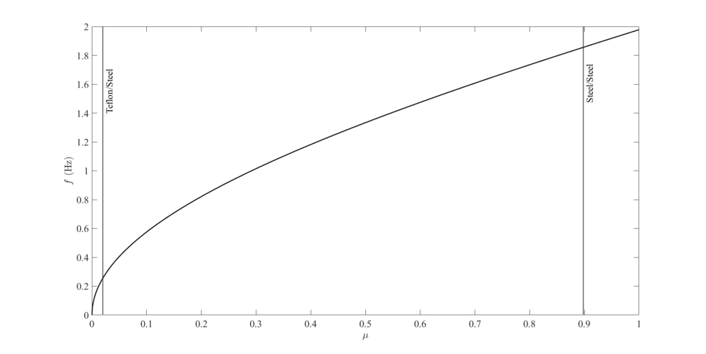
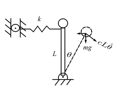
![\[V = \frac{1}{2}k(L \sin \theta)^2 - mgL(1 - \cos \theta)\]](https://engcourses-uofa.ca/wp-content/ql-cache/quicklatex.com-18e80e6ac0e6733e7d5688756e02e3ce_l3.png "Rendered by QuickLaTeX.com")
![\[T = \frac{1}{2}m(\dot{\theta L})^2\]](https://engcourses-uofa.ca/wp-content/ql-cache/quicklatex.com-5117fd68bf36cb9d0c687d19c8f56ffc_l3.png "Rendered by QuickLaTeX.com")
![\[\frac{d}{dt}(\frac{\partial L}{\partial q_i}) - \frac{\partial L}{\partial q_i} = Q_i\]](https://engcourses-uofa.ca/wp-content/ql-cache/quicklatex.com-7c40a0f01cd0f551dde9ef49f1c0986c_l3.png "Rendered by QuickLaTeX.com")
![\[mL^2 \ddot{\theta} + kL^2 \sin \theta \cos \theta - mgL \sin \theta + cL^2 \dot{\theta} = 0\]](https://engcourses-uofa.ca/wp-content/ql-cache/quicklatex.com-7307dc2ee967766593401325b3b6d3f9_l3.png "Rendered by QuickLaTeX.com")
The equilibrium configurations are:
![\[\theta _o = 0, \pi\]](https://engcourses-uofa.ca/wp-content/ql-cache/quicklatex.com-1a078f637f9eaa934fd420d05bfec71e_l3.png "Rendered by QuickLaTeX.com")
and
![\[\sin \theta _o [kL^2 \cos \theta _o - mgL] = 0\]](https://engcourses-uofa.ca/wp-content/ql-cache/quicklatex.com-967143049309d4fdf55a60f563442871_l3.png "Rendered by QuickLaTeX.com")
therefore,
![\[\cos \theta _o = \frac{mg}{kL}\]](https://engcourses-uofa.ca/wp-content/ql-cache/quicklatex.com-47e1af1e2d7de2dd6a03572b879c23ea_l3.png "Rendered by QuickLaTeX.com")
![\[V = \frac{1}{2}k(L \sin \theta)^2 - mgL(1 - cos \theta)\]](https://engcourses-uofa.ca/wp-content/ql-cache/quicklatex.com-332893cce999000151d3baeab9cbc3a9_l3.png "Rendered by QuickLaTeX.com")
![\[\begin{split} \frac{\partial V}{\partial \theta} &= kL^2 \sin \theta \cos \theta - mgL \sin \theta \\&= kL^2[\sin \theta \cos \theta - \frac{mg}{kL} \sin \theta] \\&= kL^2 \sin \theta \big( \cos \theta - \frac{mg}{kL}\big) \end{split}\]](https://engcourses-uofa.ca/wp-content/ql-cache/quicklatex.com-9f87dcca27ce33e56afefb9c907b0568_l3.png "Rendered by QuickLaTeX.com")
![\[\frac{\partial^2V}{\partial \theta^2} = k L^2 \cos \theta \left(\cos \theta - \frac{mg}{kL}\right) - kL^2\sin \theta \]](https://engcourses-uofa.ca/wp-content/ql-cache/quicklatex.com-a1e79be0cf46f89367dd62b9a21c9e85_l3.png "Rendered by QuickLaTeX.com")
At 
![\[= kL^2 [1(1-\frac{mg}{kL})]\]](https://engcourses-uofa.ca/wp-content/ql-cache/quicklatex.com-79dec0e91f4f43ea787bbb7378586631_l3.png "Rendered by QuickLaTeX.com")
 if
if  ,
, 
at 
![\[kL^2\left[\left(-1\right)\left(-1-\frac{mg}{kL}\right)\right] > 0 \]](https://engcourses-uofa.ca/wp-content/ql-cache/quicklatex.com-e2bf50f60171eeb4e5861e0408f5a5d2_l3.png "Rendered by QuickLaTeX.com")
Therefore always stable
at  when
when 
![\[\frac{\partial ^2 V}{\partial \theta ^2} = -kL^2 \sin \theta _o\]](https://engcourses-uofa.ca/wp-content/ql-cache/quicklatex.com-ad6ca5848b91785670aedd9469cb5a72_l3.png "Rendered by QuickLaTeX.com")
therefore, always unstable.
This is easy to do for a SDOF (MDOF), however for general systems it is not as straightforward. For the general case, there are mathematical techniques that are used and referred to by the work of Routh, E.J. done in ‘Rigid Dynamics’ 1897. We will consider it for the case of the ‘1 1/2” and two DOF systems only.
7.2. Mathematical Criterion of Stability
(J.P. Den Hartog, Mechanical Vibrations, 4th Ed. 1956)
For single-degree-of-freedom systems, the criterion of dynamic stability can be derived by physical rather than by mathematical means. With systems of two or three degrees of freedom, a physical conception is always very helpful but usually does not give a complete interpretation of what happens. A mathematical approach is necessary, and this involves at first the setting up of the differential equations of the problem. As long as we deal with small vibrations (and thus disregard any non-linearities that may exist), the equations are all linear and of the second order. Their solution, as usual, is found by assuming the following:
![\[x_1 = X_1e^{st}\]](https://engcourses-uofa.ca/wp-content/ql-cache/quicklatex.com-804db584cbf8d57b5dedda6575b5ce55_l3.png "Rendered by QuickLaTeX.com")
![\[x_2 = X_2e^{st} \]](https://engcourses-uofa.ca/wp-content/ql-cache/quicklatex.com-245a05c60b2828a5ce07f98efcda3143_l3.png "Rendered by QuickLaTeX.com")
![\[\vdots\]](https://engcourses-uofa.ca/wp-content/ql-cache/quicklatex.com-8bcf0b1fee7a0c2d2a81ece774534f4d_l3.png "Rendered by QuickLaTeX.com")
![\[x_n = X_ne^{st}\]](https://engcourses-uofa.ca/wp-content/ql-cache/quicklatex.com-d2e4d5baa9f1edce8ff90a729bf8e1ae_l3.png "Rendered by QuickLaTeX.com")
where is a complex number the real part of which determines the damping and the imaginary part of which is the natural frequency. Substituting into the differential equations of the free vibration transforms these equations into a set of n homogeneous, linear algebraic equations in the (complex) unknowns  . A process of algebraic elimination is then performed with the result that one equation is obtained which does not contain any of these variables. This equation, known as the “frequency equation,” is generally of the degree 2n in s. Thus, for a two-degree-of-freedom system we obtain a quartic; for a three-degree-of freedom system we obtain a sixth-degree equation, etc.
An algebraic equation of degree 2n in the variable s has 2n roots or 2n values of s. Real roots of s would lead to terms  in the solution, which rarely occur in ordinary vibrating systems. The roots of s are usually complex and then they always occur in conjugate pairs:
![\[s_1 = p_1 + jq_1\]](https://engcourses-uofa.ca/wp-content/ql-cache/quicklatex.com-e9929dd2be2c0d98737c618744f08f78_l3.png "Rendered by QuickLaTeX.com")
![\[s_2 = p_1 - jq_1\]](https://engcourses-uofa.ca/wp-content/ql-cache/quicklatex.com-257d5bbef3efa822e76829660c44548d_l3.png "Rendered by QuickLaTeX.com")
![\[s_3 = p_2 + jq_2\]](https://engcourses-uofa.ca/wp-content/ql-cache/quicklatex.com-c500b2a5b0d7d05c439a4c53c1052885_l3.png "Rendered by QuickLaTeX.com")
![\[s_4 = p_2 - jq_2\]](https://engcourses-uofa.ca/wp-content/ql-cache/quicklatex.com-ee8052d353c82daa30eba3b06a3807d9_l3.png "Rendered by QuickLaTeX.com")
The solution of the first differential equation is
![\[x_1 = C_1 e^{s_1t} + C_2 e^{s_2t} + C_3 e^{s_3t} + ...\]](https://engcourses-uofa.ca/wp-content/ql-cache/quicklatex.com-4340c7791e6c1299fd6f805fb2531aa6_l3.png "Rendered by QuickLaTeX.com")
We know that these terms can be combined by pairs as follows:
![\[C_1e^{s_1t} + C_2e^{s_2t} = e^{p_1t}(A \sin q_1t + B \cos q_1t)\]](https://engcourses-uofa.ca/wp-content/ql-cache/quicklatex.com-ace4ac8e34e39524ce56717d41b916a4_l3.png "Rendered by QuickLaTeX.com")
so that the imaginary part of s is the frequency, and the real part of determines the rate of damping. If the real parts of all the values of s are negative, the system is dynamically stable; but if the real part of any one of the values of s is positive, the system is dynamically unstable.
Therefore the stability can be determined by an examination of the signs of the real parts of the solutions of the frequency equation. It is not necessary to solve the equation, because certain rules exist by which from an inspection of the coefficients of the equation a conclusion regarding the stability or instability can be drawn. These rules, which were given by Routh in 1877, are rather complicated for frequency equations of higher degree, but for the most practical cases (third and fourth degree) they are sufficiently simple.
Let us consider first the cubic equation
![\[s^3 + A_2s^2 + A_1s + A_0 = 0 \quad (\star)\]](https://engcourses-uofa.ca/wp-content/ql-cache/quicklatex.com-28a4e15f3dcb6fe3a37572d3cf1f9fdd_l3.png "Rendered by QuickLaTeX.com")
(7.4) which occurs in the case of two degrees of freedom where one mass or spring is zero (in a sense one and one-half degrees of freedom)If its roots are  and
and  ,
,  can be written
![\[(s-s_1)\cdot (s-s_2) \cdot (s-s_3) = 0\]](https://engcourses-uofa.ca/wp-content/ql-cache/quicklatex.com-7cd1b1816d75cc675d1459b7116f3399_l3.png "Rendered by QuickLaTeX.com")
or, worked out,
![\[s^3 - (s_1 + s_2 + s_3)s^2 + (s_1s_2 + s_1s_3+s_2s_3)s - s_1s_2s_3 = 0 \]](https://engcourses-uofa.ca/wp-content/ql-cache/quicklatex.com-31a5d61df762f4f41124920c2b7c2876_l3.png "Rendered by QuickLaTeX.com")
A comparison shows the following:
![\[A_2 = -(s_1 + s_2 + s_3)\]](https://engcourses-uofa.ca/wp-content/ql-cache/quicklatex.com-6939e49f7d645b9393b737c76e4407e5_l3.png "Rendered by QuickLaTeX.com")
![\[A_1 = s_1s_2 + s_1s_3 + s_2s_3 \qquad (\star \star) \]](https://engcourses-uofa.ca/wp-content/ql-cache/quicklatex.com-890cea07ac790b2967ff34544dcc8f95_l3.png "Rendered by QuickLaTeX.com")
![\[A_0 = -s_1s_2s_3\]](https://engcourses-uofa.ca/wp-content/ql-cache/quicklatex.com-710b89891c3736052f9ea9b05838c6c0_l3.png "Rendered by QuickLaTeX.com")
One of the three roots of a cubic equation must always be real, and the other two are either real or conjugate complex. Separating the roots  into their real and imaginary parts, we may write
![\[s_1 = p_1\]](https://engcourses-uofa.ca/wp-content/ql-cache/quicklatex.com-df33e9a8388886f7945f28313e0ccf19_l3.png "Rendered by QuickLaTeX.com")
![\[s_2 = p_2 + jq_2\]](https://engcourses-uofa.ca/wp-content/ql-cache/quicklatex.com-4520ca3beec4b55d14e9c9ba38d2da77_l3.png "Rendered by QuickLaTeX.com")
![\[s_3 = p_2 - jq_2\]](https://engcourses-uofa.ca/wp-content/ql-cache/quicklatex.com-8017d282612f94272af51e30dc730c4e_l3.png "Rendered by QuickLaTeX.com")
Substituted into  this leads to the following:
![\[A_2 = -(p_1 + 2p_2)\]](https://engcourses-uofa.ca/wp-content/ql-cache/quicklatex.com-c82a469ab6cc0f84aa5fcf8be5bf8192_l3.png "Rendered by QuickLaTeX.com")
![\[A_1 = 2p_1p_2 + p_2^2 + q_2^2\]](https://engcourses-uofa.ca/wp-content/ql-cache/quicklatex.com-380e3dc9e5ca0bdb80a07ac870346b3b_l3.png "Rendered by QuickLaTeX.com")
![\[A_0 = -p_1(p_2^2 + q_2^2)\]](https://engcourses-uofa.ca/wp-content/ql-cache/quicklatex.com-41d2cabb2cd700f07dbc5beb36417c5e_l3.png "Rendered by QuickLaTeX.com")
The criterion of stability is that both  and
and  be negative. It is seen in the first place that all coefficients
  , and
, and  must be positive, because, if any one of them were negative, the above requires that either or , or both and , must be positive. This requirement can be proved to hold for higher degree equations as well. Hence a frequency equation of any degree with one or more negative coefficients determines an unstable motion.
Granted that the coefficients,  and
and  are all positive, the third equation requires that be negative. No information about is available as yet. However, on the boundary between stability and instability, must pass from a positive to a negative value through zero. Make = 0 and we can derive the following:
![\[A_2 = -p_1\]](https://engcourses-uofa.ca/wp-content/ql-cache/quicklatex.com-91848ec4145a49ad7e85d9e21e9fb8de_l3.png "Rendered by QuickLaTeX.com")
![\[A_1 = q_2^2\]](https://engcourses-uofa.ca/wp-content/ql-cache/quicklatex.com-58357b12c965af90a88a0e278896e19a_l3.png "Rendered by QuickLaTeX.com")
![\[A_0 = -p_1q_2^2\]](https://engcourses-uofa.ca/wp-content/ql-cache/quicklatex.com-ab5e70d3b809d26f9932a71ce6572354_l3.png "Rendered by QuickLaTeX.com")
These relations must be satisfied on the boundary of stability. By eliminating and we find
![\[A_0 = A_1A_2\]](https://engcourses-uofa.ca/wp-content/ql-cache/quicklatex.com-18c4271c33cdef92f7a81dddc87ccff5_l3.png "Rendered by QuickLaTeX.com")
We do not know yet on which side of this relation stability exists. That can be found in the simplest manner by trying out one particular case. For example let  and
and  , which obviously is a stable solution. Substitution gives
![\[A_2 = 3, A_1 = 4, A_0 = 2\]](https://engcourses-uofa.ca/wp-content/ql-cache/quicklatex.com-5696bfed879fa37c87f4607c9185f4a6_l3.png "Rendered by QuickLaTeX.com")
so that
![\[A_o < A_1A_2\]](https://engcourses-uofa.ca/wp-content/ql-cache/quicklatex.com-fff65a57f4719ed79377c0a9f915432b_l3.png "Rendered by QuickLaTeX.com")
The complete criterion for stability of the cubic is that all coefficients A are positive and that
![\[A_1A_2 > A_0\]](https://engcourses-uofa.ca/wp-content/ql-cache/quicklatex.com-1961cf0f84d9dba4742d4bb81c9d45c7_l3.png "Rendered by QuickLaTeX.com")
Next consider the quartic
![\[s^4 + A_3s^3 + A_2s^2 + A_1s + A_0 = 0 \]](https://engcourses-uofa.ca/wp-content/ql-cache/quicklatex.com-dbacf1538f452e80f82ede4b008cf2fc_l3.png "Rendered by QuickLaTeX.com")
for which the procedure is similar. Since a quartic can be resolved into two quadratic factors, we may write for the roots:
![\[s_2 = p_1-jq_1\]](https://engcourses-uofa.ca/wp-content/ql-cache/quicklatex.com-253cfb9ed07e9fdea67c92a611d97bf0_l3.png "Rendered by QuickLaTeX.com")
![\[s_4 - p_2 - jq_2\]](https://engcourses-uofa.ca/wp-content/ql-cache/quicklatex.com-0c85c0549fba65f0436dcb027256a841_l3.png "Rendered by QuickLaTeX.com")
and substitite in, which leads to:
![\[A_3 = -2(p_1 + p_2)\]](https://engcourses-uofa.ca/wp-content/ql-cache/quicklatex.com-3294d145b2a240da9e8dc0d2addf1b8b_l3.png "Rendered by QuickLaTeX.com")
![\[A_2 = p_1^2 + p_2^2 + q_1^2 + q_2^2 + 4p_1p_2\]](https://engcourses-uofa.ca/wp-content/ql-cache/quicklatex.com-28ce5339fa5f02d6a7d679d20f1e1fb1_l3.png "Rendered by QuickLaTeX.com")
![\[A_1 = -2p_1 \cdot (p_2^2 + q_2^2) - 2p_2(p_1^2 + q_1^2)\]](https://engcourses-uofa.ca/wp-content/ql-cache/quicklatex.com-c42f0b5853b93c451a9573054962bc93_l3.png "Rendered by QuickLaTeX.com")
![\[A_0 = (p_1^2 + q_1^2) \cdot (p_2^2 + q_2^2)\]](https://engcourses-uofa.ca/wp-content/ql-cache/quicklatex.com-3534e90cde76b1279a4e3532b5d9f5ba_l3.png "Rendered by QuickLaTeX.com")
The requirement for stability is that both and be negative. Substitution of negative values of and makes all four A‘s positive, so that the first requirement for stability is that all coefficients A be positive. Granted that this is so, the first equation requires that at least one of the quantities or be negative. Let be negative. We still need another requirement to make also negative. On the boundary between stability and instability, = 0, which substituted in gives:
![\[A_3 = -2p_1\]](https://engcourses-uofa.ca/wp-content/ql-cache/quicklatex.com-63b6e9da6ff4f74ca6d91cb814e956ee_l3.png "Rendered by QuickLaTeX.com")
![\[A_2 = p_1^2 + q_1^2 + q_2^2\]](https://engcourses-uofa.ca/wp-content/ql-cache/quicklatex.com-6b4fa9158ea5cd79c659f73727809225_l3.png "Rendered by QuickLaTeX.com")
![\[A_1 = -2p_1q_2^2\]](https://engcourses-uofa.ca/wp-content/ql-cache/quicklatex.com-7e9ca0d3d1471cbe10bb7235c1934962_l3.png "Rendered by QuickLaTeX.com")
![\[A_0 = (p_1^2 + q_1^2)q_2^2\]](https://engcourses-uofa.ca/wp-content/ql-cache/quicklatex.com-1c96173d0f6c683772692342c050fae9_l3.png "Rendered by QuickLaTeX.com")
being four equations in the three variables 
Elimination of these variables leads to a relations between the  ‘s:
‘s:
![\[ A_1A_2A_3 = A_1^2 + A_3^2A_0 \]](https://engcourses-uofa.ca/wp-content/ql-cache/quicklatex.com-b943cfea1b6250a4432d78f26aa020f9_l3.png "Rendered by QuickLaTeX.com")
To find out on which side of this equality stability exists, we try out a simple stable case, for example:
![\[ s_\text{1,2} = -1 \pm j, \quad s_\text{3,4} = -2 \pm 2j \]](https://engcourses-uofa.ca/wp-content/ql-cache/quicklatex.com-ee1989fcbdecd8626035bc0a4b1eb2c8_l3.png "Rendered by QuickLaTeX.com")
Which, on substitution, gives:
![\[ A_3 = 6,\ A_2 = 18,\ A_1 = 24,\ A_0 = 16 \]](https://engcourses-uofa.ca/wp-content/ql-cache/quicklatex.com-c90fe40222ec451d465de94af00360e5_l3.png "Rendered by QuickLaTeX.com")
So that  . Thus, the complete criterion for stability of the quartic (7.10) is that all coefficients are positive and that:
![\[ A_1A_2A_3 > A_1^2 + A_2^3A_0 \]](https://engcourses-uofa.ca/wp-content/ql-cache/quicklatex.com-f4e8893956a01aefcaaa440311cba2c7_l3.png "Rendered by QuickLaTeX.com")
Systems with three degrees of freedom generally have a sextic for their frequency equation and in degenerated cases, a quintic. In such cases, there are three real parts of the roots , and besides the requirements of positive signs for all coefficients A, there are two other requirements, each of which is rather lengthy. For further information, the reader is referred to the original work of Routh.
Example
Investigate the stability of motion of a pendulum of length and mass rotating with constant angular velocity about its vertical axis.
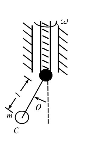
Assume during the steady state rotation about the vertical axis as small angle is given to the pendulum and  is the corresponding variation in the angular velocity. Use the Lagrangian formulation to determine the equations of motion.
![\[ v_c^2 = \ell^2 \theta^2 (\omega + \dot{\phi})^2 + \ell_2 (\dot{\theta})^2 \]](https://engcourses-uofa.ca/wp-content/ql-cache/quicklatex.com-453a0faa07d2dc5e7d64c351086eaf19_l3.png "Rendered by QuickLaTeX.com")
Therefore:
![\[ T = \frac{1}{2} m \ell^2 (\omega^2 \theta^2 + (\dot{\theta})^2) \quad \text{(neglecting } (\dot{\phi})^2 \text{ as small)} \]](https://engcourses-uofa.ca/wp-content/ql-cache/quicklatex.com-c253770c838aa502c95d443e8568bdfe_l3.png "Rendered by QuickLaTeX.com")
![\[ V = \frac{1}{2}mg\theta^2 \quad \text{(} 1 - \cos \theta \approx \theta^2 \text{ for } \theta << 1 \text{)} \]](https://engcourses-uofa.ca/wp-content/ql-cache/quicklatex.com-afe345debe4b0ca5aae9b3002b8b06a8_l3.png "Rendered by QuickLaTeX.com")
![\[ \Big[ \frac{d}{dt} \Big(\frac{\partial L}{\partial \dot{q}_i}\Big) - \frac{\partial L}{\partial q_i} = 0 \Big] \]](https://engcourses-uofa.ca/wp-content/ql-cache/quicklatex.com-235cff3c7888801f000a6365addd1e8a_l3.png "Rendered by QuickLaTeX.com")
Thus:
![\[ m \ell^2 \ddot{\theta} - m \ell^2 \omega^2 \theta + mg \theta = 0 \]](https://engcourses-uofa.ca/wp-content/ql-cache/quicklatex.com-64c2fa21efccdfafe5b948c6ac5ee119_l3.png "Rendered by QuickLaTeX.com")
![\[ \ddot{\theta} + \Big(\frac{g}{\ell} - \omega^2\Big) \theta = 0 \]](https://engcourses-uofa.ca/wp-content/ql-cache/quicklatex.com-99fb4ca7cfc42a860e0e482c991c6c9b_l3.png "Rendered by QuickLaTeX.com")
If there was viscous damping  , the equation would be:
![\[ \ddot{\theta} + 2c\dot{\theta} + \Big(\frac{g}{\ell} - \omega^2\Big) \theta = 0 \]](https://engcourses-uofa.ca/wp-content/ql-cache/quicklatex.com-659a14455dc9fcee449f5414d8c11670_l3.png "Rendered by QuickLaTeX.com")
Therefore, assuming  with
with  :
:
![\[ s^2 + 2cs + p^2 = 0\]](https://engcourses-uofa.ca/wp-content/ql-cache/quicklatex.com-3baa9c94305b2b215046b1f867adc3d0_l3.png "Rendered by QuickLaTeX.com")
![\[ s = -c \pm \sqrt{c^2 - p^2} \]](https://engcourses-uofa.ca/wp-content/ql-cache/quicklatex.com-7db5a60d467e1acc8ddc4cf232dd7d7a_l3.png "Rendered by QuickLaTeX.com")
So that if  is negative, one of the roots is positive and the motion is unstable.
Example
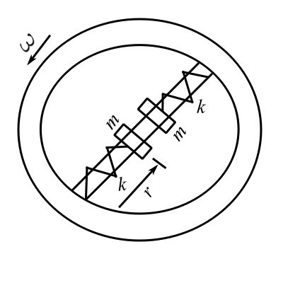
Look at the stability of the steady rotation of a horizontal flywheel carrying two masses attached to hub by springs and free to slide along the spokes. If  is the moment of inertia of the flywheel, is the angular velocity, and
  is the upstretched lengths of the springs. Let
  be the small change in
  and the small change in .
![\[ T = \frac{1}{2} (\omega + \dot{\phi})^2 + m[(r+x)^2(\omega + \dot{\phi})^2 + \dot{x}^2] \]](https://engcourses-uofa.ca/wp-content/ql-cache/quicklatex.com-a5d4de346973590023d56f5c3018db09_l3.png "Rendered by QuickLaTeX.com")
![\[ V = k(r - a + x)^2 - k(r-a)^2 \]](https://engcourses-uofa.ca/wp-content/ql-cache/quicklatex.com-a0e4f53bcf7482fc69bd053d8e3a9127_l3.png "Rendered by QuickLaTeX.com")
Using Lagrange’s equations and omitting terms of higher order in the small quantities leaves:
![\[ (J+ 2mr^2) \ddot{\phi} + 4mr\omega\dot{x}^2 = 0\]](https://engcourses-uofa.ca/wp-content/ql-cache/quicklatex.com-16c7f4e2505bcb4a158813a230e8a1a5_l3.png "Rendered by QuickLaTeX.com")
![\[ m\ddot{x} - m\omega^2(r+x) - 2m\omega r\dot{\phi} + k(r-a+x) = 0 \]](https://engcourses-uofa.ca/wp-content/ql-cache/quicklatex.com-e2c4e0d934e5c68524acf279b6c05029_l3.png "Rendered by QuickLaTeX.com")
But the equilibrium configuration when  . Therefore:
![\[ m\omega^2s = k(s-a) \quad (*) \]](https://engcourses-uofa.ca/wp-content/ql-cache/quicklatex.com-a90b21fd893da069b5da9319b855bd07_l3.png "Rendered by QuickLaTeX.com")
If we put  with
with  , we obtain:
![\[ (J + 2mr^2)sC_1 + 4mr\omega s C_2 = 0\]](https://engcourses-uofa.ca/wp-content/ql-cache/quicklatex.com-238646d3ff3f9bccb16f0c6e9ed9820f_l3.png "Rendered by QuickLaTeX.com")
![\[ -2m \omega s C_1 + (ms^2 - m\omega^2 + k)C_2 = 0\]](https://engcourses-uofa.ca/wp-content/ql-cache/quicklatex.com-e98b2d9439a43d807ffeba50edbd59d6_l3.png "Rendered by QuickLaTeX.com")
For a non-trivial solution:
![\[ (J + 2mr^2)s(ms^2 - m\omega^2 + k) + 8m^2r^2\omega^2s = 0 \]](https://engcourses-uofa.ca/wp-content/ql-cache/quicklatex.com-8e6b43362dc8be15439ad58182d51960_l3.png "Rendered by QuickLaTeX.com")
This equation will have a positive root if:
![\[ -m\omega^2 + k + \frac{8mr^2\omega^2}{J + 2mr^2} < 0\]](https://engcourses-uofa.ca/wp-content/ql-cache/quicklatex.com-3c8819c7a457787bcbbe1363b5d516bc_l3.png "Rendered by QuickLaTeX.com")
![\[\omega^2\Big(1- \frac{8mr^2}{J + 2mr^2}\Big) > \frac{k}{m}\]](https://engcourses-uofa.ca/wp-content/ql-cache/quicklatex.com-bdb4811b26bd1d6283629d93aa539679_l3.png "Rendered by QuickLaTeX.com")