
Advanced Dynamics and Vibrations: Continuous Systems
Continuous Systems and Waves
The difference between discrete and continuous systems is that we go from a finite number to an infinite number of degrees of freedom. Mathematically, this means that the equations of motion go from ordinary to partial differential equations.
We will consider a number of continuous systems including strings, rods, and beams.
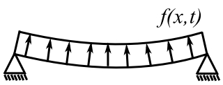
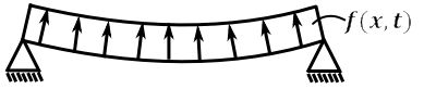
First, consider a flexible string of mass per unit length  and stretched under a tension
  .
.
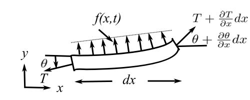
Where  is the shape. The string could also be loaded laterally with a
  .
.
For small angles,  . Thus:
![\[ \begin{split} + \uparrow \sum F_y &= f(x,t) dx + \Big(T + \frac{\partial T}{\partial x} dx \Big) \Big( \frac{\partial y}{\partial x} + \frac{\partial^2 y(x)}{\partial x^2} dx \Big) - T \frac{\partial y}{\partial x} \\&= \rho dx\frac{\partial^2 y}{\partial t^2} \end{split} \]](https://engcourses-uofa.ca/wp-content/ql-cache/quicklatex.com-08484b870895e18c8d90f1d0477234af_l3.png "Rendered by QuickLaTeX.com")
![\[ \frac{\partial T}{\partial x} \frac{\partial y}{\partial x} dx + T \frac{\partial^2 y}{\partial x^2} dx + f(x,t)dx = \rho dx\frac{\partial^2 y}{\partial t^2} \]](https://engcourses-uofa.ca/wp-content/ql-cache/quicklatex.com-6395a0029e778ce2472f0a47f2989529_l3.png "Rendered by QuickLaTeX.com")
Therefore:
![\[ \frac{\partial}{\partial x}\Big[ T(x) \frac{\partial y}{\partial x} \Big] + f(x,t) = \rho(x)\frac{\partial^2 y}{\partial t^2} \]](https://engcourses-uofa.ca/wp-content/ql-cache/quicklatex.com-d590322268bfaef4cb9788918e71ceb2_l3.png "Rendered by QuickLaTeX.com")
As we did for discrete systems, we look for the so-called synchronized motions and start with the free-vibration case. Therefore, assume:
![\[ y(x,t) = Y(x)G(t) \]](https://engcourses-uofa.ca/wp-content/ql-cache/quicklatex.com-a5073db1d47d13eca8853d485a602b8d_l3.png "Rendered by QuickLaTeX.com")
We are looking for special cases where all the particles are described by  and this varies in time.
![\[ \begin{split} \frac{1}{\rho (x) Y(x)} &= \frac{d}{dx} \Big[T(x) \frac{dY}{dx}\Big] \\&= \frac{1}{G(t)} \frac{d^2 G(t)}{dt} \end{split} \]](https://engcourses-uofa.ca/wp-content/ql-cache/quicklatex.com-ddf166e2de03268489b993827165c39e_l3.png "Rendered by QuickLaTeX.com")
As the LHS is a function of only  and the RHS is a function of only time, each side must be equal to a constant. Therefore, without loss of generality, set:
![\[ -p^2 = \frac{1}{G(t)} \frac{d^2 G(t)}{d t^2} \]](https://engcourses-uofa.ca/wp-content/ql-cache/quicklatex.com-f0d4728d61058561f310f14179bad7f9_l3.png "Rendered by QuickLaTeX.com")
Therefore, the solution for  is:
is:
![\[ G(t) = C \cos (pt - \phi) \]](https://engcourses-uofa.ca/wp-content/ql-cache/quicklatex.com-b7dbff2f657e6aa75277e19101f966f9_l3.png "Rendered by QuickLaTeX.com")
Where  and
and  are constants. This leaves an O.D.E.
![\[ \frac{d}{dx}\Big[ T(x) \frac{d Y(x)}{dx} \Big] + p^2 \rho(x)Y(x) = 0 \quad (*) \]](https://engcourses-uofa.ca/wp-content/ql-cache/quicklatex.com-9dbc9b586f850b8530f9f75bd61d92a9_l3.png "Rendered by QuickLaTeX.com")
instead of an algebraic problem that we had in the discrete case. Solving this, yields the natural frequencies and the mode shapes.
![\[ [p_1,Y_1],\ [p_2,Y_2]\ .... \]](https://engcourses-uofa.ca/wp-content/ql-cache/quicklatex.com-3a40acf8696bfe74337ca2c05ab0d003_l3.png "Rendered by QuickLaTeX.com")
However, there are an infinite number.
We can normalize the eigenfunctions, as they satisfy the orthogonality conditions.
![\[ \int_{0}^{L} \rho(x) Y_r(x) Y_s(x) dx = \delta rs \]](https://engcourses-uofa.ca/wp-content/ql-cache/quicklatex.com-16e716a03b15963ae3e61dc3f03ccb48_l3.png "Rendered by QuickLaTeX.com")
We will also see that
![\[ \int_{0}^{L} T(x) \frac{d Y_r}{d x} \frac{d Y_s}{d x} dx = p_r^2 \delta rs \]](https://engcourses-uofa.ca/wp-content/ql-cache/quicklatex.com-673f588bf7f7d2a2d7e5edf01b21a25f_l3.png "Rendered by QuickLaTeX.com")
And this leads to an expansion theorem analogous to what we saw in the discrete case. This is the normal mode solution and therefore not the only solution of the partial differential equation. We will consider the other types of solutions.
Consider an example of a uniform string, where  (constant) and
  . Note that:
![\[ \beta^2 \equiv \frac{p^2 \rho}{T} \]](https://engcourses-uofa.ca/wp-content/ql-cache/quicklatex.com-2b26cd7968c4730e3b68230ed1ce2921_l3.png "Rendered by QuickLaTeX.com")
The equation (*) becomes:
![\[ \frac{d^2 Y}{d x^2} + \beta^2 Y(x) = 0 \]](https://engcourses-uofa.ca/wp-content/ql-cache/quicklatex.com-dc6cad9bfd55cb52d68e69a3df384b72_l3.png "Rendered by QuickLaTeX.com")
Thus:
![\[ Y(x) = A \sin \beta x + B \cos \beta x \]](https://engcourses-uofa.ca/wp-content/ql-cache/quicklatex.com-36c86022e49e9a6e9b5002f1c24c91f4_l3.png "Rendered by QuickLaTeX.com")
Where  and
and  are found from the boundary conditions.
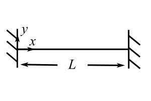
![\[y(0,t) = 0,\ y(L,t) = 0 \]](https://engcourses-uofa.ca/wp-content/ql-cache/quicklatex.com-37bb3af01e7149fe00fc1140a25e6693_l3.png "Rendered by QuickLaTeX.com")
Therefore:
![\[ Y(0) = 0,\ Y(L) = 0\]](https://engcourses-uofa.ca/wp-content/ql-cache/quicklatex.com-e3dd5c5ba349e4df3c98125691030599_l3.png "Rendered by QuickLaTeX.com")
![\[ B = 0 \]](https://engcourses-uofa.ca/wp-content/ql-cache/quicklatex.com-105dc5a3160e668f1aae904646d38e9c_l3.png "Rendered by QuickLaTeX.com")
Therefore:
![\[ \begin {split} Y(L) &= A \sin \beta L \\&= 0 \text{ (characteristic equation)} \end{split} \]](https://engcourses-uofa.ca/wp-content/ql-cache/quicklatex.com-dc09e7d1b7566b790df98c23128bbe66_l3.png "Rendered by QuickLaTeX.com")
![\[ \beta L = n\pi \]](https://engcourses-uofa.ca/wp-content/ql-cache/quicklatex.com-11dcc7437634b626ad6d9246639bf9bc_l3.png "Rendered by QuickLaTeX.com")
![\[ p_n \sqrt{\frac{\rho}{T}}L = n\pi \]](https://engcourses-uofa.ca/wp-content/ql-cache/quicklatex.com-da41a7e5addaedb0e97397f73f8c3cb2_l3.png "Rendered by QuickLaTeX.com")
![\[p_n = \frac{n\pi}{L} \sqrt{\frac{T}{\rho}} \]](https://engcourses-uofa.ca/wp-content/ql-cache/quicklatex.com-9fe94f7f0cf538a31ecfdaf77f2ddb5e_l3.png "Rendered by QuickLaTeX.com")
![\[ \sqrt{\frac{T}{\rho}} \equiv c \]](https://engcourses-uofa.ca/wp-content/ql-cache/quicklatex.com-831cc049cd1e5e29ac9a52d830c7123c_l3.png "Rendered by QuickLaTeX.com")
Thus:
![\[p_n = \frac{n\pi c}{L} \]](https://engcourses-uofa.ca/wp-content/ql-cache/quicklatex.com-f9aae357672edbedf19ebc1040c2b865_l3.png "Rendered by QuickLaTeX.com")
We can have other boundary conditions, for example
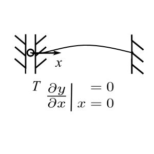
![\[ T\frac{\partial y}{\partial x}|_{x=0} = 0 \]](https://engcourses-uofa.ca/wp-content/ql-cache/quicklatex.com-dbe9bc203b3dacca469a7f80a6618ed0_l3.png "Rendered by QuickLaTeX.com")
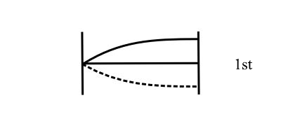
For pin supports, the mode shapes are simply:
![\[ A_n \sin \frac{n\pi x}{L} \]](https://engcourses-uofa.ca/wp-content/ql-cache/quicklatex.com-01a4852e841684960933335a68fe8cfd_l3.png "Rendered by QuickLaTeX.com")
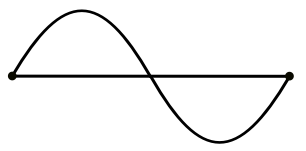
1st Mode
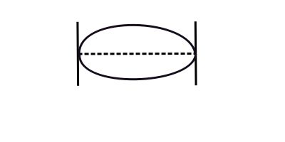
![\[p_1 = \frac{\pi c}{L} \]](https://engcourses-uofa.ca/wp-content/ql-cache/quicklatex.com-8f3f5d957210acda5c806d49399dc860_l3.png "Rendered by QuickLaTeX.com")
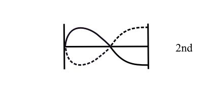
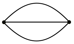
2nd Mode
![\[p_2 = \frac{2 \pi c}{L} \]](https://engcourses-uofa.ca/wp-content/ql-cache/quicklatex.com-a026ff2bf4022225fda40477967daee0_l3.png "Rendered by QuickLaTeX.com")
Check the orthogonality condition.
![\[ \int_{0}^{L} \rho(x) Y_r(x) Y_s(x) dx = \delta rs \]](https://engcourses-uofa.ca/wp-content/ql-cache/quicklatex.com-7b7c25a280fb76e22393858a27cae940_l3.png "Rendered by QuickLaTeX.com")
If :
![\[ \begin{split} \rho \int_{0}^L A_r^2 \sin^2 \frac{r \pi x}{L} dx &= \frac{A^2_r \rho}{2} \int_{0}^L \Big(1 - \cos \frac{2r\pi x}{L} \Big) dx \\&= \frac{A_r^2 \rho}{2} \Big\{\Big[L - \frac{L}{2\pi r} \sin \frac{2 r \pi x}{L}\Big]_0^L \Big\} \\&= \frac{A_r^2 \rho L}{2} \\&= 1 \end{split} \]](https://engcourses-uofa.ca/wp-content/ql-cache/quicklatex.com-4a77edddf890397526c85229dfbe902b_l3.png "Rendered by QuickLaTeX.com")
Therefore:
![\[ A_r = \sqrt{\frac{2}{\rho L}},\ Y_r(x) = \sqrt{\frac{2}{\rho L}} \sin \frac{r \pi x}{L} \]](https://engcourses-uofa.ca/wp-content/ql-cache/quicklatex.com-cf77f36cc8a0a2f8f3a49e3439f44c71_l3.png "Rendered by QuickLaTeX.com")
If  :
:
![\[ \int_0^L \rho Y_r Y_S dx = \frac{2}{L} \int_0^L \sin \frac{r \pi x}{L} \sin \frac{s \pi x}{L} dx \]](https://engcourses-uofa.ca/wp-content/ql-cache/quicklatex.com-2622a66bfc4b5d98ad64065112f7d3e8_l3.png "Rendered by QuickLaTeX.com")
Use the identity ![\sin \alpha \sin \beta = \frac{1}{2} [ \cos ( \alpha - \beta) - \cos (\alpha + \beta) ]](https://engcourses-uofa.ca/wp-content/ql-cache/quicklatex.com-8b50e7d03efcf3672cf42bd13bcba830_l3.png "Rendered by QuickLaTeX.com") :
:
![\[ \begin{split} &= \frac{1}{L} \int_0^L \Big( \cos (r-s) \frac{\pi x}{L} - \cos (r+s) \frac{\pi x}{L} \Big) dx \\&= 0 \end{split} \]](https://engcourses-uofa.ca/wp-content/ql-cache/quicklatex.com-71b70ca80cdf65947ba68a94d02cbb7c_l3.png "Rendered by QuickLaTeX.com")
If we consider the other boundary condition:
![\[ \frac{ dY } {dx}\Big|_{x=L} = 0,\ Y(x) = A \sin \beta x \]](https://engcourses-uofa.ca/wp-content/ql-cache/quicklatex.com-ddaa90ab3c2c6b70050f9f32b9d6cd40_l3.png "Rendered by QuickLaTeX.com")
![\[ \frac{ dY } {dx} = A\beta \cos \beta x \]](https://engcourses-uofa.ca/wp-content/ql-cache/quicklatex.com-3c13a52d86bff476d4feda78e57568be_l3.png "Rendered by QuickLaTeX.com")
Therefore:
![\[ 0 = \cos \beta L \Rightarrow \beta L = \Big(2n + 1\Big) \frac{\pi}{2} \qquad n = 0, 1, 2, \ldots \]](https://engcourses-uofa.ca/wp-content/ql-cache/quicklatex.com-74daf0c2d9dce0616c3d102ec610ab1f_l3.png "Rendered by QuickLaTeX.com")
![\[ Y(x) = A_n \sin (2n+1) \frac{\pi}{2} \frac{x}{L} \]](https://engcourses-uofa.ca/wp-content/ql-cache/quicklatex.com-4a42c4e207c97410410f0f300a74ef06_l3.png "Rendered by QuickLaTeX.com")
1st Mode
![\[p_1 = \frac{\pi c}{2L}, \ \sin \frac{\pi x}{2L} \]](https://engcourses-uofa.ca/wp-content/ql-cache/quicklatex.com-eb4862690f913d65bf3616456fcefbb9_l3.png "Rendered by QuickLaTeX.com")
2nd Mode
![\[p_2 = \frac{3 \pi c}{2L}, \ \sin \frac{3 \pi x}{2L} \]](https://engcourses-uofa.ca/wp-content/ql-cache/quicklatex.com-dcc4c26032192850a5fc62a5c81a7c41_l3.png "Rendered by QuickLaTeX.com")
Consider a more general solution of the equation when is constant:
![\[ \frac{\partial^2 y}{\partial x^2} = \frac{\rho}{T} \frac{\partial^2 y}{\partial t^2} \]](https://engcourses-uofa.ca/wp-content/ql-cache/quicklatex.com-7815f3d5e250772f2538269dee299f61_l3.png "Rendered by QuickLaTeX.com")
And since we defined  :
:
![\[ \frac{\partial^2 y}{\partial x^2} = \frac{1}{c^2} \frac{\partial^2 y}{\partial t^2} \]](https://engcourses-uofa.ca/wp-content/ql-cache/quicklatex.com-86da4e038bc979cac92f5dae63f27847_l3.png "Rendered by QuickLaTeX.com")
If we take any functions of the form:
![\[ y = F(ct - x) + G(ct + x) \]](https://engcourses-uofa.ca/wp-content/ql-cache/quicklatex.com-1f64fa4b40708a954607577cfc642a95_l3.png "Rendered by QuickLaTeX.com")
Where  and
and  . Then
  and
and  both satisfy the differential equation. Thus:
![\[ \begin{split} \frac{\partial y}{\partial x} &= \frac{\partial F}{\partial \gamma} \frac{\partial \gamma}{\partial x} + \frac{\partial G}{\partial \epsilon}\frac{\partial \epsilon}{\partial x}\\&= -\frac{\partial F}{\partial \gamma} + \frac{\partial G}{ \partial \epsilon} \end{split} \]](https://engcourses-uofa.ca/wp-content/ql-cache/quicklatex.com-56e5ac2dde8f2db596e888921b444812_l3.png "Rendered by QuickLaTeX.com")
![\[ \frac{\partial^2 y}{\partial x^2} = \frac{\partial^2 F}{\partial \gamma^2} + \frac{\partial^2 G}{\partial \epsilon^2} \]](https://engcourses-uofa.ca/wp-content/ql-cache/quicklatex.com-a886f370f45991463e8fb76bd7fd2ce0_l3.png "Rendered by QuickLaTeX.com")
![\[ \frac{\partial y}{\partial t} = c\Big(\frac{\partial F}{\partial \gamma} + \frac{\partial G}{\partial \epsilon}\Big) \]](https://engcourses-uofa.ca/wp-content/ql-cache/quicklatex.com-2ead704b65beb0c535897fb0841a9204_l3.png "Rendered by QuickLaTeX.com")
![\[ \frac{\partial^2 y}{\partial t^2} = c^2 \Big(\frac{\partial^2 F}{\partial \gamma^2} + \frac{\partial^2 G}{\partial \epsilon^2} \Big) \]](https://engcourses-uofa.ca/wp-content/ql-cache/quicklatex.com-615ac481cdf410cedc4e831814fc0be4_l3.png "Rendered by QuickLaTeX.com")
Therefore, both and satisfy the differential equation. Consider a physical interpretation of and . This leads to the idea of waves on the string. In this case, the particle motion is perpendicular to the wave motion (transverse wave) as opposed to longitudinal waves.
Consider any function that might be:

If the  , then the value of must be the same. Therefore,
  . Thus:
![\[ \begin{split} c &= \frac{x_1 - x_o}{t_1 - t_o} \\&= \frac{\Delta x}{\Delta t} \end{split} \]](https://engcourses-uofa.ca/wp-content/ql-cache/quicklatex.com-16d2fb77fe3771b5cab6d69b3f460432_l3.png "Rendered by QuickLaTeX.com")
This is a velocity and  is called the wave speed for a wave moving in the positive direction.
Similarly for  , we can show that the wave is moving in the negative direction. This can be used in several applications as:
![\[ c = \sqrt{\frac{T}{\rho}} \]](https://engcourses-uofa.ca/wp-content/ql-cache/quicklatex.com-05e2c4eced21658eb1661f68d833a089_l3.png "Rendered by QuickLaTeX.com")
Therefore, if we measure , we can determine !
What happens when this waves hits a boundary? As the disturbance reaches an end point it is reflected and the incident plus reflected wave must add to zero to satisfy the boundary condition.
As a result, there is a 180 degree phase shift and a wave of  becomes
  .
.
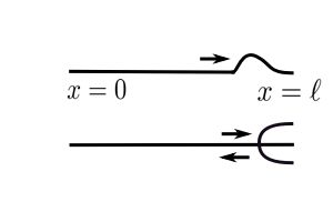
So that the sum at  is zero. As the velocity is , the time for the round trip is
  .
.
One of the functions that is a positive travelling wave  is a harmonic function –
  . Imagine a wave emanating from the origin in this form.
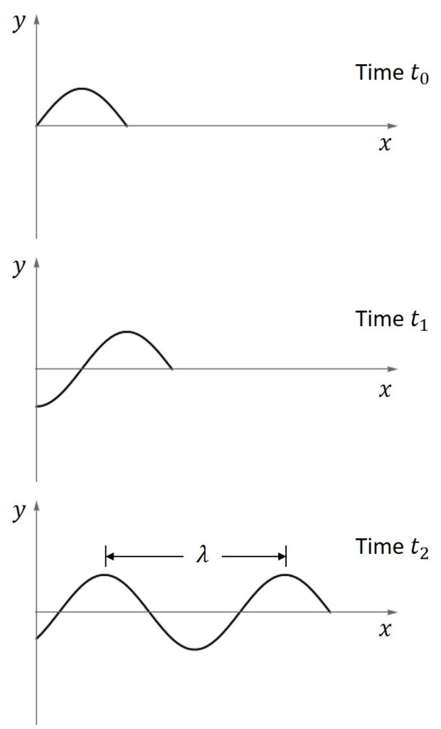
![\[\begin{split}\lambda &= c \cdot \text{period of oscillation} \\ &= c\tau = c\left(\frac{1}{f}\right) \\ \therefore c &= f\lambda \end{split} \]](https://engcourses-uofa.ca/wp-content/ql-cache/quicklatex.com-af895b685f9c272ce2075cd465de3335_l3.png "Rendered by QuickLaTeX.com")
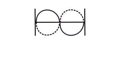
We can then see the vibration occurs when the positive wave and negative wave at the same time.
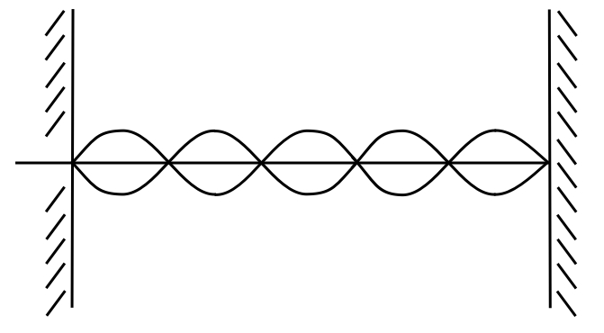
This is then a standing wave.
This is what Naum Gabo called the “Kinetic Art” in 1919!
Example
Consider a guy wire 1 000 ft long made of 1 1/4″ diameter bridge strand cable that weighs 2.50 lbs/ft with breaking strength of 130 000 lbs, working at 50 000 lbs.
![\[ \begin{split} c &= \sqrt{\frac{(50000)(32.2)}{2.50}} \\&= 802 \text{ ft/sec} \end{split} \]](https://engcourses-uofa.ca/wp-content/ql-cache/quicklatex.com-d28223249abe08b7825debf04e905871_l3.png "Rendered by QuickLaTeX.com")
Therefore:
![\[ \begin{split} \frac{2 \ell}{c} &= \frac{2000}{802} \\&\approx 2.5 \text{ seconds} \end{split} \]](https://engcourses-uofa.ca/wp-content/ql-cache/quicklatex.com-683bfee19bcb0a5867fc15a8bd454842_l3.png "Rendered by QuickLaTeX.com")
Note: Analogous to the string is the longitudinal and torsional vibration of a bar. Each differential equation looks the same however the speed has a different interpretation.
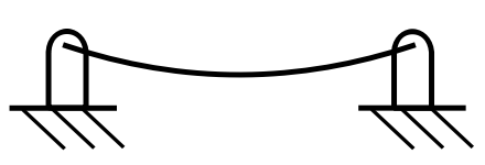
Example: CBC Tower in Calgary
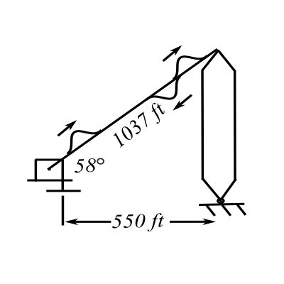
![\[ 1 \frac{1}{8}"\ \phi \text{ Bridge Strand} \]](https://engcourses-uofa.ca/wp-content/ql-cache/quicklatex.com-b07844c2299ab363811e0a37671e9a87_l3.png "Rendered by QuickLaTeX.com")
![\[T @ 10^{\circ} C = 23400 \text{ lbs} \]](https://engcourses-uofa.ca/wp-content/ql-cache/quicklatex.com-e00902613edde55922bf1dd72e1d387a_l3.png "Rendered by QuickLaTeX.com")
![\[\text{Cable Weighs } 2.61 \text{ lbs/ft} \]](https://engcourses-uofa.ca/wp-content/ql-cache/quicklatex.com-410701e7297202fadc5fbf0f102ee566_l3.png "Rendered by QuickLaTeX.com")
![\[ c^2 = \frac{(23400)(32.2)}{2.61} \Rightarrow c = 537 \text{ ft/sec (366 MPH)} \]](https://engcourses-uofa.ca/wp-content/ql-cache/quicklatex.com-e8725f5d246a6d65f0102736860133fe_l3.png "Rendered by QuickLaTeX.com")
Therefore, the time to travel  ft:
ft:
![\[ \begin{split} t &= \frac{1037(2)}{537} \\&= 3.86 \text{ seconds} \end{split} \]](https://engcourses-uofa.ca/wp-content/ql-cache/quicklatex.com-fc251e1db2e7026d28ee744dd37d0402_l3.png "Rendered by QuickLaTeX.com")
On site measurements of wind-induced cable vibration showed a standing wave pattern
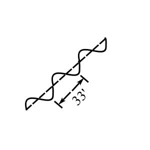
Which mode of vibration is this?
![\[ \begin{split} f_1 &= \frac{c}{2L} \\&= \frac{1}{3.86} \\&= 0.26 \text{ Hz} \end{split} \]](https://engcourses-uofa.ca/wp-content/ql-cache/quicklatex.com-3fd0a945682dbe4c35d6ffa6d490e1a3_l3.png "Rendered by QuickLaTeX.com")
![\[ \begin{split} f_2 &= \frac{2c}{2L} \\&= 0.58 \text{ Hz} \end{split} \]](https://engcourses-uofa.ca/wp-content/ql-cache/quicklatex.com-26134ed356097471a43359b7b682fd3f_l3.png "Rendered by QuickLaTeX.com")
![\[ f_n = 8.7 \text{ Hz (measured)} \]](https://engcourses-uofa.ca/wp-content/ql-cache/quicklatex.com-6271ca3bc681499e4adfa74e2cfd4683_l3.png "Rendered by QuickLaTeX.com")
Where  ?
?
![\[\begin{split} f_n &= \frac{nc}{2L} \\&= 8.7 \end{split} \]](https://engcourses-uofa.ca/wp-content/ql-cache/quicklatex.com-b19a8a376efc122474a8302762b6e7a1_l3.png "Rendered by QuickLaTeX.com")
![\[\begin{split} n &= 8.7(3.86) \\n &= 33 \sim 34 \text{ mode!} \end{split} \]](https://engcourses-uofa.ca/wp-content/ql-cache/quicklatex.com-691708c600c466065023de4412e851d3_l3.png "Rendered by QuickLaTeX.com")
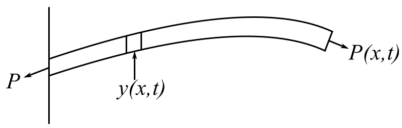
Longitudinal Vibration of a Bar
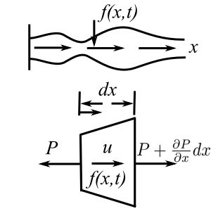
Assuming a 1-D stress field:
![\[ P = EA\frac{\partial u}{\partial x} \]](https://engcourses-uofa.ca/wp-content/ql-cache/quicklatex.com-d552bb79e43654bc6d67e6cd91f5d86f_l3.png "Rendered by QuickLaTeX.com")
![\[ \Big(P + \frac{\partial P}{\partial x} dx \Big) + f(x,t) dx - P = \rho A dx \frac{\partial^2 u}{\partial t^2} \]](https://engcourses-uofa.ca/wp-content/ql-cache/quicklatex.com-531615076b7c781d712e840997bc60d9_l3.png "Rendered by QuickLaTeX.com")
Therefore:
![\[ \frac{\partial}{\partial x} \Big(EA \frac{\partial u}{\partial x} \Big) + f(x,t) = \rho(x) A(x) \frac{\partial^2 u}{\partial t^2} \]](https://engcourses-uofa.ca/wp-content/ql-cache/quicklatex.com-544c6d2a1ab131c7f7183e4d2ed3d701_l3.png "Rendered by QuickLaTeX.com")
For a uniform bar:
![\[EA \frac{\partial^2 u}{\partial x^2} = \rho A \frac{\partial^2 u}{\partial t^2} \]](https://engcourses-uofa.ca/wp-content/ql-cache/quicklatex.com-9c30af505592ef8d43840e3157ba5890_l3.png "Rendered by QuickLaTeX.com")
The equation is similar to the string:
![\[ \frac{ \partial^2 u}{\partial x^2} = \frac{1}{c_A^2} \frac{\partial^2 u}{\partial t^2} \]](https://engcourses-uofa.ca/wp-content/ql-cache/quicklatex.com-318b6539059cd8de251f8d65ae7d239f_l3.png "Rendered by QuickLaTeX.com")
For Steel:
![\[ \begin{split} c_A &= \sqrt{\frac{E}{\rho}} \\&= \sqrt{\frac{30 \cdot 10^6 \cdot 386}{286}} \\&= 16860 \text{ ft/s} \end{split} \]](https://engcourses-uofa.ca/wp-content/ql-cache/quicklatex.com-2141edc4b9237cb716caeb116166ce78_l3.png "Rendered by QuickLaTeX.com")
Where the subscript indicates axial wave velocity.
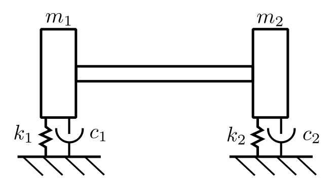
Again we can have boundary conditions which are similar to the string.
With:

– damping coefficient
Therefore:
![\[ m_2\ddot{u} \Big|_{x=\ell} = -EA\frac{\partial u}{\partial x} (\ell, t) - ku(\ell, t) - C \frac{\partial u}{\partial t} (\ell t) \]](https://engcourses-uofa.ca/wp-content/ql-cache/quicklatex.com-9b6ca0d92b59df77c7f83e23c12b6f50_l3.png "Rendered by QuickLaTeX.com")
Is the general boundary condition. The solution follows the same procedure as the string:
![\[ u(x,t) = X(x)T(t) \]](https://engcourses-uofa.ca/wp-content/ql-cache/quicklatex.com-7f551af2d90c2740a036f51c950ee83f_l3.png "Rendered by QuickLaTeX.com")
![\[\begin{split} c_A^2 \frac{X''(x)}{X(x)} &= \frac{T''(t)}{T(t)} \\&= -p^2 \end{split} \]](https://engcourses-uofa.ca/wp-content/ql-cache/quicklatex.com-332fe8f8717fb11ea4adcdc708901f76_l3.png "Rendered by QuickLaTeX.com")
Therefore:
![\[ X''(x) + \frac{p^2}{c_A^2}X(x) = 0 \]](https://engcourses-uofa.ca/wp-content/ql-cache/quicklatex.com-e6c96179b4c3f439e68acdc9fff33b23_l3.png "Rendered by QuickLaTeX.com")
![\[ X(x) = D \sin \frac{p}{c_A} x + B \cos \frac{p}{c_A} x \]](https://engcourses-uofa.ca/wp-content/ql-cache/quicklatex.com-1f586190655a794f86f4fd4d30e67b6a_l3.png "Rendered by QuickLaTeX.com")
If at  ,
,  , therefore:
Thus:
![\[ u(x,t) = D \sin \frac{p}{c_A} x \cos( pt - \phi) \]](https://engcourses-uofa.ca/wp-content/ql-cache/quicklatex.com-6623ea9ee404887bb39ea65f12fc30e2_l3.png "Rendered by QuickLaTeX.com")
![\[ \ddot{u}(x,t) = -p^2 D \sin \frac{p}{c_A} x \cos(pt-\phi)\]](https://engcourses-uofa.ca/wp-content/ql-cache/quicklatex.com-088853a6e2a3ec66f12f7dbb9f7eb56f_l3.png "Rendered by QuickLaTeX.com")
Consider the free boundary condition at  :
:
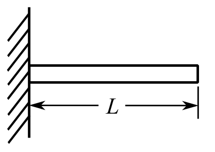
![\[ u(0,t) = 0,\ P(L,t) = 0 \Rightarrow \frac{\partial u}{\partial t}(L,t) = 0 \]](https://engcourses-uofa.ca/wp-content/ql-cache/quicklatex.com-629e3a681e1ddcf9f28dd6063a13992d_l3.png "Rendered by QuickLaTeX.com")
![\[ X(x) = D \sin \frac{p}{c_A} x + B \cos \frac{p}{c_A}x \]](https://engcourses-uofa.ca/wp-content/ql-cache/quicklatex.com-25c2cd18e43003577600776353de955c_l3.png "Rendered by QuickLaTeX.com")
![\[X(0) = 0 \Rightarrow B = 0 \]](https://engcourses-uofa.ca/wp-content/ql-cache/quicklatex.com-29b13034c7749ac03abb372addb63fc6_l3.png "Rendered by QuickLaTeX.com")
![\[ \frac{\partial u}{\partial x}\Big|_{x=L} = 0 \Rightarrow \frac{dX}{dx} \Big|_{x=L} = 0 \]](https://engcourses-uofa.ca/wp-content/ql-cache/quicklatex.com-d49bc537ba8a0644db5bc04f52b1c107_l3.png "Rendered by QuickLaTeX.com")
![\[ D \frac{p}{c_A} \cos \frac{p}{c_A} L = 0 \]](https://engcourses-uofa.ca/wp-content/ql-cache/quicklatex.com-3414903b826c50f7b48363c745244924_l3.png "Rendered by QuickLaTeX.com")
Therefore:
![\[ p \frac{L}{c_A} = (2n + 1) \frac{\pi}{2} \quad n = 0,1,2,... \]](https://engcourses-uofa.ca/wp-content/ql-cache/quicklatex.com-168a338003603bbfbb30bddf1ce6714b_l3.png "Rendered by QuickLaTeX.com")
![\[ p_1 \frac{L}{c_A} = \frac{\pi}{2} \]](https://engcourses-uofa.ca/wp-content/ql-cache/quicklatex.com-2000dc53eeb787bed631b43ea6af15da_l3.png "Rendered by QuickLaTeX.com")
![\[ p_1 = \frac{c_A}{L} \frac{\pi}{2} \]](https://engcourses-uofa.ca/wp-content/ql-cache/quicklatex.com-e7ada03dfb0d2bb57bbbace5cc15c982_l3.png "Rendered by QuickLaTeX.com")
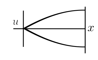
Therefore:
![\[ \begin{split} \text{for } p_1 &\Rightarrow D \sin\left( \frac{\pi c_A x}{2 L c_A}\right) = X_1 \quad \text{First Mode} \\X_1 &= D \sin\left( \frac{\pi x}{2L}\right) \end{split} \]](https://engcourses-uofa.ca/wp-content/ql-cache/quicklatex.com-c37d19d4a10c7e871af7435d5b8f34b4_l3.png "Rendered by QuickLaTeX.com")
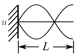
For the 2nd Mode:
![\[ \frac{p_2 L}{c_A} = \frac{3\pi}{2} \]](https://engcourses-uofa.ca/wp-content/ql-cache/quicklatex.com-18174f349fb96ed3bd334a3e1b2bfe0d_l3.png "Rendered by QuickLaTeX.com")
![\[ p_2 = \frac{3}{2} \pi \frac{c_A}{L} \]](https://engcourses-uofa.ca/wp-content/ql-cache/quicklatex.com-e9c51650bc0e3d77b7cf8be9715ac3c9_l3.png "Rendered by QuickLaTeX.com")
![\[ X_2 = D \sin\left( \frac{3}{2} \pi \frac{c_A}{L} \frac{x}{c_A}\right) = D \sin\left( \frac{3 \pi x}{2L}\right) \]](https://engcourses-uofa.ca/wp-content/ql-cache/quicklatex.com-79469e757be7b2cecd24619552fc20fd_l3.png "Rendered by QuickLaTeX.com")
We can now consider a mass  at the end of the bar. The boundary condition is then:
![\[ m_2 \frac{d^2 u}{dx^2}\Big|_{x=L} = -EA \frac{\partial u}{\partial x} (L, t) \]](https://engcourses-uofa.ca/wp-content/ql-cache/quicklatex.com-a627ffcd25a8b4251ed07430f5812b65_l3.png "Rendered by QuickLaTeX.com")
Therefore:
![\[ -EAD \frac{p}{c_A} \cos \frac{p}{c_A} x\Big|_{x=L} = -m_2p^2D \sin \frac{p}{c_A}x\Big|_{x=L} \]](https://engcourses-uofa.ca/wp-content/ql-cache/quicklatex.com-e5189d78bb79d23a23e284c9017beb56_l3.png "Rendered by QuickLaTeX.com")
![\[ \frac{EA}{m_2c_Ap} = \tan \frac{p}{c_A} L \]](https://engcourses-uofa.ca/wp-content/ql-cache/quicklatex.com-847479acde5a404ebe16ab9c0e4ced48_l3.png "Rendered by QuickLaTeX.com")
Where  and
and  .
.
![\[ \frac{c_A^2 \rho A}{m_2c_Ap} = \tan \frac{p}{c_A} L \]](https://engcourses-uofa.ca/wp-content/ql-cache/quicklatex.com-2046b4d90014e953f5a01c09332ef8a2_l3.png "Rendered by QuickLaTeX.com")
But  – mass of rod. Therefore:
![\[ \frac{pAL}{m_2} \frac{c_A}{pL} = \tan \frac{p}{c_A} L \]](https://engcourses-uofa.ca/wp-content/ql-cache/quicklatex.com-56ddf4d1b7e3956d40c3d6bfbfad8a57_l3.png "Rendered by QuickLaTeX.com")
![\[ \frac{m}{m_2} = \gamma \tan \gamma \]](https://engcourses-uofa.ca/wp-content/ql-cache/quicklatex.com-5b9a1b1737c2f76ad94bb47387036908_l3.png "Rendered by QuickLaTeX.com")
Where  . We can consider the mass of a “spring” in the calculation of the system natural frequency.
![\[ \begin{split} \gamma &= \frac{pL}{c_A} \\&= pL\sqrt{\frac{\rho}{E}} \end{split} \]](https://engcourses-uofa.ca/wp-content/ql-cache/quicklatex.com-e028b7bf2e0dd04de4bae359200d78ab_l3.png "Rendered by QuickLaTeX.com")
To put this in a form we recognize, recall:
![\[ \frac{P}{A} = E\frac{\Delta L}{L} \]](https://engcourses-uofa.ca/wp-content/ql-cache/quicklatex.com-d997b51f3a28a5a8d364678a418bfdf6_l3.png "Rendered by QuickLaTeX.com")
Therefore:
![\[ \begin{split} P &= \frac{EA}{L} \Delta L \\&= "k"\Delta L \end{split} \]](https://engcourses-uofa.ca/wp-content/ql-cache/quicklatex.com-665fd4439cf9bdcc30130792849dab86_l3.png "Rendered by QuickLaTeX.com")
Therefore:
![\[ \begin{split} \gamma &= pL\sqrt{\frac{A\rho}{kL}} \\&= p \sqrt{\frac{A \rho L}{k}} \\&= p\sqrt{\frac{m}{k}} \end{split} \]](https://engcourses-uofa.ca/wp-content/ql-cache/quicklatex.com-b787db8f052024e7abea3dce0e7dc9ae_l3.png "Rendered by QuickLaTeX.com")
Where  is the mass of the rod or spring. As a result, we must solve this transcendental equation to find
  for a given
  ratio.
Example
![\[ \frac{m}{m_2} = \frac{1}{2} \Rightarrow \gamma = 0.6534 \qquad \text{(for lowest }p, p_1\text{)}\]](https://engcourses-uofa.ca/wp-content/ql-cache/quicklatex.com-f8fc29e620f59e2941d551f7fcba03ec_l3.png "Rendered by QuickLaTeX.com")
![\[\begin{split} p_1 &= 0.6534\sqrt{\frac{k}{m}} \\&= 0.6534 \sqrt{\frac{2k}{m_2}} \\&= 0.924\sqrt{\frac{k}{m_2}} \end{split} \]](https://engcourses-uofa.ca/wp-content/ql-cache/quicklatex.com-aa16cae4270392a5a05e359e647aa5e7_l3.png "Rendered by QuickLaTeX.com")
If we used the rule of thumb:
![\[ \begin{split} p_1 &= \sqrt{\frac{k}{m_2 + \frac{m}{3}}} \\&= \sqrt{\frac{k}{m_2 + \frac{m_2}{6}}} \\&= \sqrt{ \frac{6}{7}\frac{k}{m_2}} \\&= 0.926\sqrt{\frac{k}{m_2}} \end{split} \]](https://engcourses-uofa.ca/wp-content/ql-cache/quicklatex.com-8cdf3a5bf1fc177333131f84f79d9ff3_l3.png "Rendered by QuickLaTeX.com")
If  , then:
![\[ \gamma = 0.8603 \]](https://engcourses-uofa.ca/wp-content/ql-cache/quicklatex.com-37f0acab9001590c204f085f6beccea6_l3.png "Rendered by QuickLaTeX.com")
![\[ p_1 = 0.860\sqrt{\frac{k}{m}} \qquad (m_2 = m)\]](https://engcourses-uofa.ca/wp-content/ql-cache/quicklatex.com-1772e1e6c5d80a7548c7bd2bb355484c_l3.png "Rendered by QuickLaTeX.com")
Using R.O.T:
![\[\begin{split} p_1 &= \sqrt{\frac{3}{4} \frac{k}{m_2}} \\&= 0.866\sqrt{\frac{k}{m}} \end{split} \qquad (m_2 = m)\]](https://engcourses-uofa.ca/wp-content/ql-cache/quicklatex.com-cce03f26e50bbf5ca6d75d1e9da5fa1f_l3.png "Rendered by QuickLaTeX.com")
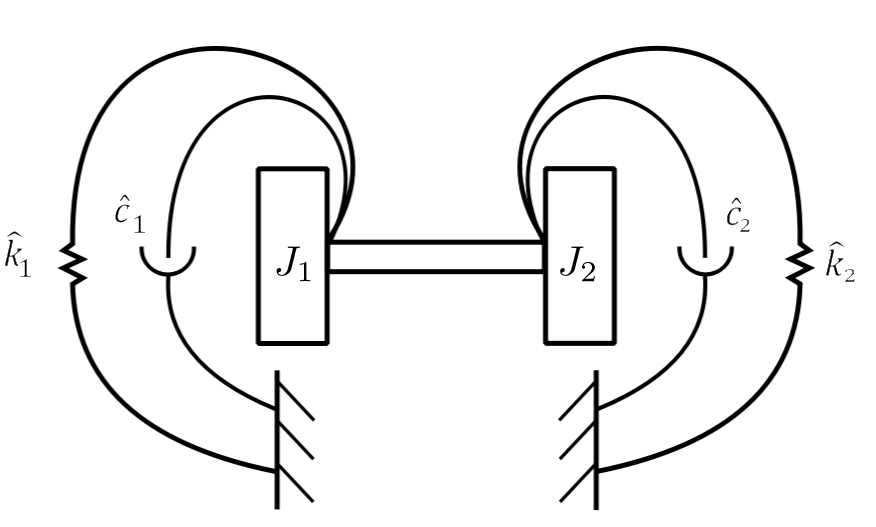
Torsional Vibration of Shafts & Rods
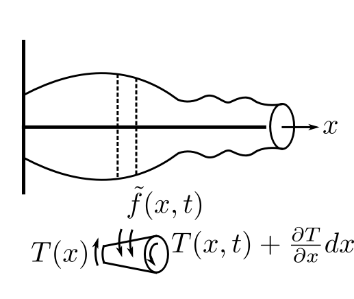
We assume that  is the polar second moment of area of the x-section.
  is the moment of inertia (polar) per unit length of the rod, where
  is the mass density.
![\[T = \mu I \frac{\partial \theta}{\partial x}\]](https://engcourses-uofa.ca/wp-content/ql-cache/quicklatex.com-482374d9db5eabcfdc0d925a7833a02b_l3.png "Rendered by QuickLaTeX.com")
The equation of motion is
![\[\frac{\partial}{\partial x}[\mu I(x) \frac{\partial \theta}{\partial x}] + \tilde{f} (x,t) = J_o dx \frac{\partial ^{2} \theta}{\partial t^{2}}\]](https://engcourses-uofa.ca/wp-content/ql-cache/quicklatex.com-e6866979a257a20877ae16bfecc6361f_l3.png "Rendered by QuickLaTeX.com")
if we consider a uniform rod for free vibration
![\[\mu I \frac{\partial ^{2} \theta}{\partial x^{2}} = \rho I \frac{\partial ^{2} \theta}{\partial t^{2}}\]](https://engcourses-uofa.ca/wp-content/ql-cache/quicklatex.com-657cd1ce861c6fb95b2a7efb33239d77_l3.png "Rendered by QuickLaTeX.com")
![\[\frac{\partial ^{2} \theta}{\partial x^{2}} = \frac{\rho}{\mu} \frac{\partial ^{2} \theta}{\partial t^{2}}\]](https://engcourses-uofa.ca/wp-content/ql-cache/quicklatex.com-8dc2464ff3729de295825a04cf49d91b_l3.png "Rendered by QuickLaTeX.com")
which is again the wave equation, therefore
![\[\theta (x,t) = \left(A \cos p \frac{x}{\tilde{c}} + B \sin p \frac{x}{\tilde{c}}\right)\cos\left(pt-\phi\right)\]](https://engcourses-uofa.ca/wp-content/ql-cache/quicklatex.com-c34175404f3010918e3b158f3085fdd5_l3.png "Rendered by QuickLaTeX.com")
where
![\[\begin{split} \tilde{c} &= \sqrt{\frac{\mu}{\rho}} \\&= \sqrt{\frac{E}{2(1+\nu) \rho}} \\& \approx 0.62 C_A \end{split}\]](https://engcourses-uofa.ca/wp-content/ql-cache/quicklatex.com-61b92fde21ad1c39402b4bd639d9609d_l3.png "Rendered by QuickLaTeX.com")
We can proceed in a completely analogous manner to the axial vibrations
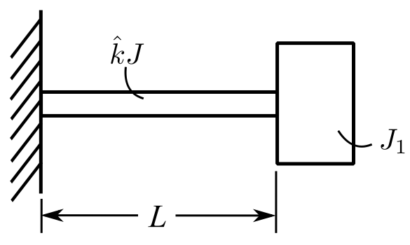
The torsional stiffness  ,
,  , therefore
![\[\begin{split} \frac{\rho}{\mu} &= \frac{J/LI}{\hat{k} L/I} \\&= \frac{J}{\hat{k} L^{2}}\end{split}\]](https://engcourses-uofa.ca/wp-content/ql-cache/quicklatex.com-26601f7d1f25f856d59ef8fc56af9efd_l3.png "Rendered by QuickLaTeX.com")
Define  where
where  is the total moment of inertia of the rod and
  is the total torsional stiffness
![\[\theta (x,t) = \left(A \cos \frac{\gamma x}{L} + B \sin \frac{\gamma x}{L}\right) \cos (pt + \phi) \]](https://engcourses-uofa.ca/wp-content/ql-cache/quicklatex.com-f45cb8b9c9826d4270c9083a8074e2ca_l3.png "Rendered by QuickLaTeX.com")
again we can solve the boundary value problem
The solution is again:
![\[\gamma \tan \gamma = \frac{J}{J_1}\]](https://engcourses-uofa.ca/wp-content/ql-cache/quicklatex.com-3d72fb1083549128ca30d451ecd24cd1_l3.png "Rendered by QuickLaTeX.com")
if 
![\[\gamma ^{2} \approx \frac{J}{J_1}\]](https://engcourses-uofa.ca/wp-content/ql-cache/quicklatex.com-c9a960af624c58b215adbd74e6237e2c_l3.png "Rendered by QuickLaTeX.com")
![\[p^{2} \frac{J}{\hat{k}} = \frac{J}{J_1}\]](https://engcourses-uofa.ca/wp-content/ql-cache/quicklatex.com-3a16e3966abb11a4a79a0084e57e979e_l3.png "Rendered by QuickLaTeX.com")
![\[p^{2} \approx \frac{\hat{k}}{J_1}\]](https://engcourses-uofa.ca/wp-content/ql-cache/quicklatex.com-32e6014b799ca42400aa62b86740588c_l3.png "Rendered by QuickLaTeX.com")
Bending Vibrations
The three problems discussed above are all of exactly the same form, the wave equation with two boundary conditions. For the bar in flexure, the bvp is a 4th order d.e.
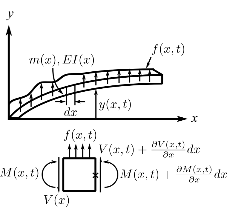
we neglect the rotation of the element in the deformation and we neglect the shear deformation with respect to the bending deformation. (We will relax these restrictions later.)
![\[\begin{split} + \uparrow \sum F_y &= f(x,t)dx - V(x) + V(x,t) + \frac{\partial V}{\partial x}dx \\&= m(x) \frac{\partial ^{2} y}{\partial t^{2}} \end{split}\]](https://engcourses-uofa.ca/wp-content/ql-cache/quicklatex.com-dbf8a12d420997e0ef03923e403dd652_l3.png "Rendered by QuickLaTeX.com")
Since we neglect the rotary inertia
![\[\begin{split} \circlearrowleft + \sum M_x &= 0 \\&= M(x,t) + \frac{\partial M}{\partial x}dx - M(x,t) + V(x)dx + f(x,t) dx \frac{dx}{2} \end{split}\]](https://engcourses-uofa.ca/wp-content/ql-cache/quicklatex.com-40de2bb5b7b10ba41e0177c8960ef6ef_l3.png "Rendered by QuickLaTeX.com")
![\[\frac{\partial M}{\partial x} + V(x) = 0 \]](https://engcourses-uofa.ca/wp-content/ql-cache/quicklatex.com-ae1d36b173e8cbb6d1b44ca0a625c03b_l3.png "Rendered by QuickLaTeX.com")
![\[-\frac{\partial ^{2} M}{\partial x^{2}} + f(x,t) = m(x) \frac{\partial ^{2} y}{\partial t^{2}}, 0<x<L\]](https://engcourses-uofa.ca/wp-content/ql-cache/quicklatex.com-60989c8a93d53b8dcf4a55c77963bebd_l3.png "Rendered by QuickLaTeX.com")
but the constitutive law gives
![\[M(x,t) = EI(x) \frac{\partial ^{2} y}{\partial x^{2}}\]](https://engcourses-uofa.ca/wp-content/ql-cache/quicklatex.com-d7c4fd2b23a39b720f2ea0304f9904b0_l3.png "Rendered by QuickLaTeX.com")
Therefore
![\[-\frac{\partial ^{2}}{\partial x^{2}}\bigg(EI(x) \frac{\partial ^{2} y}{\partial x^{2}}\bigg) + f(x,t) = m(x) \frac{\partial ^{2} y}{\partial t^{2}}\]](https://engcourses-uofa.ca/wp-content/ql-cache/quicklatex.com-dddc0957acc850fc013890de2aac9499_l3.png "Rendered by QuickLaTeX.com")
The boundary conditions are:
1.Clamped ends at x=0
![\[y(0,t) = 0 , \frac{\partial y}{\partial x}\bigg|_{x=0} = 0\]](https://engcourses-uofa.ca/wp-content/ql-cache/quicklatex.com-0bf1c4eb089412ceba2f7dd4ab4f6c1e_l3.png "Rendered by QuickLaTeX.com")
2.Hinged end
![\[y(0,t) = 0 , EI(x)\frac{\partial ^{2} y}{\partial x^{2}}(x,t) \bigg|_{x=0} = 0 \]](https://engcourses-uofa.ca/wp-content/ql-cache/quicklatex.com-a0fe31ae00a747a22d527c69d30e1499_l3.png "Rendered by QuickLaTeX.com")
3.Free end
![\[EI(x)\frac{\partial ^{2} y}{\partial x^{2}}(x,t) \bigg|_{x=0} = 0, \frac{\partial }{\partial x}\bigg(EI(x) \frac{\partial ^{2} y}{\partial x^{2}}\bigg)\bigg|_{x=0} = 0\]](https://engcourses-uofa.ca/wp-content/ql-cache/quicklatex.com-27b8d0a5b41f2b1341c1622ffb4679e4_l3.png "Rendered by QuickLaTeX.com")
We divide these boundary conditions into geometric and natural boundary conditions.
Geometric:
![\[y(0,t) = 0, \frac{\partial y}{\partial x}\bigg|_{x=0} = 0\]](https://engcourses-uofa.ca/wp-content/ql-cache/quicklatex.com-5a53325f188719d1913a83cad123090c_l3.png "Rendered by QuickLaTeX.com")
Natural:
(This difference is important when dealing with approximate solutions.) Again we look for synchronous solutions.
![\[y(x,t) = Y(x)G(t)\]](https://engcourses-uofa.ca/wp-content/ql-cache/quicklatex.com-ac2803b094c275fc11b89bf88f65f776_l3.png "Rendered by QuickLaTeX.com")
This again leads to
![\[G(t) = C \cos(pt - \phi)\]](https://engcourses-uofa.ca/wp-content/ql-cache/quicklatex.com-8ce0f89e66fd7c52884aa38482534aa7_l3.png "Rendered by QuickLaTeX.com")
and an o.d.e
![\[\frac{d^{2}}{dx^{2}} \bigg(EI(x) \frac{d ^{2} Y(x)}{d x^{2}}\bigg) = p^{2}m(x)Y(x), 0<x<L \qquad (*)\]](https://engcourses-uofa.ca/wp-content/ql-cache/quicklatex.com-e1739ea55bb4cda3d1ac323073a8c013_l3.png "Rendered by QuickLaTeX.com")
This is an eigenvalue problem.
Additional b.c.’s
![\[\frac{\partial }{\partial x}\bigg(EI \frac{\partial ^{2} y}{\partial x^{2}}\bigg) = a[ky + c \frac{\partial y}{\partial t} + m \frac{\partial ^{2} w}{\partial t^{2}}]\]](https://engcourses-uofa.ca/wp-content/ql-cache/quicklatex.com-23e1ba2b920ff267078bdd230715da08_l3.png "Rendered by QuickLaTeX.com")
where  for the right end, and
  for the left end
![\[EI \frac{\partial ^{2} y}{\partial x^{2}} = a\bigg[\hat{k}\frac{\partial y}{\partial x} + \hat{c}\frac{\partial ^{2} y}{\partial x \partial t} + J_o \frac{\partial ^{3} w}{\partial x \partial t^{2}}\bigg]\]](https://engcourses-uofa.ca/wp-content/ql-cache/quicklatex.com-61f847f2675dc2bb6c6503fa4583840a_l3.png "Rendered by QuickLaTeX.com")
This gives b.c.’s for a torsional spring damper & rotational inertia.
There is no general solution to (*) but there are solutions for certain special cases. For example, consider a uniform bar:
![\[\frac{d^{4}Y(x)}{dx^{4}} - \frac{p^{2}m}{EI} Y(x) = 0\]](https://engcourses-uofa.ca/wp-content/ql-cache/quicklatex.com-63e90a42b9882c907fbc7c4cf6d88377_l3.png "Rendered by QuickLaTeX.com")
let 
The general solution of this equation is 
![\[e^{sx}(s^{4} - \beta ^{4}) = 0\]](https://engcourses-uofa.ca/wp-content/ql-cache/quicklatex.com-d407673e988c5d240632b1cdc7c0f7ad_l3.png "Rendered by QuickLaTeX.com")
Therefore:
![\[(s^{2}+\beta ^{2})(s^{2}-\beta ^{2}) = 0\]](https://engcourses-uofa.ca/wp-content/ql-cache/quicklatex.com-803aaf75568f7b5c096d402d6d4737af_l3.png "Rendered by QuickLaTeX.com")
![\[s = \beta, -\beta, i \beta, -i \beta\]](https://engcourses-uofa.ca/wp-content/ql-cache/quicklatex.com-2840fdb7841a3c4b51b1adc03d28274e_l3.png "Rendered by QuickLaTeX.com")
Therefore:
![\[Y(x) = Ce^{\beta x} + De^{-\beta x} + Ee^{i \beta x} + Fe^{-i \beta x}\]](https://engcourses-uofa.ca/wp-content/ql-cache/quicklatex.com-84ae21c5e42f6923f6d707cea1a7fe80_l3.png "Rendered by QuickLaTeX.com")
or equivalently
![\[Y(x) = C_1 \sin \beta x + C_2 \cos \beta x + C_3 \sinh \beta x + C_4 \cosh \beta x\]](https://engcourses-uofa.ca/wp-content/ql-cache/quicklatex.com-de134b58077701ff115e6e312e2dabc3_l3.png "Rendered by QuickLaTeX.com")
Where  must be determined from the boundary conditions.
If we consider a simply supported beam then
![\[\textcircled{1} y(0,t) = 0\]](https://engcourses-uofa.ca/wp-content/ql-cache/quicklatex.com-15cb744c835ed2170f7f7e10eafae77b_l3.png "Rendered by QuickLaTeX.com")
![\[\textcircled{2} \frac{\partial ^{2} y}{\partial x^{2}}(0,t) = 0\]](https://engcourses-uofa.ca/wp-content/ql-cache/quicklatex.com-34c6aae2226225ca089ccea9d9b36a17_l3.png "Rendered by QuickLaTeX.com")
![\[\textcircled{3} y(L,t) = 0\]](https://engcourses-uofa.ca/wp-content/ql-cache/quicklatex.com-9767856ab95fb460386f11f653fc7eb3_l3.png "Rendered by QuickLaTeX.com")
![\[\textcircled{4} \frac{\partial ^{2} y}{\partial x^{2}}(L,t) = 0\]](https://engcourses-uofa.ca/wp-content/ql-cache/quicklatex.com-fbe2bfe8dcfdedb8bdbed6449bf53220_l3.png "Rendered by QuickLaTeX.com")
 gives:
![\[C_2 + C_4 = 0\]](https://engcourses-uofa.ca/wp-content/ql-cache/quicklatex.com-bf395a08455213c1aaeb5b5f6db6b0b6_l3.png "Rendered by QuickLaTeX.com")
 gives:
![\[\beta ^{2} (-C_2 + C_4) = 0\]](https://engcourses-uofa.ca/wp-content/ql-cache/quicklatex.com-d3d42f9568463fe856bbbd7453657ee6_l3.png "Rendered by QuickLaTeX.com")
Therefore:
![\[C_2 = C_4 = 0\]](https://engcourses-uofa.ca/wp-content/ql-cache/quicklatex.com-c90eed491b414473969def027f544924_l3.png "Rendered by QuickLaTeX.com")
 gives:
![\[C_1 \sin \beta L + C_3 \sinh \beta L = 0\]](https://engcourses-uofa.ca/wp-content/ql-cache/quicklatex.com-7cca25e5dfb9b85b319b62d703cfa699_l3.png "Rendered by QuickLaTeX.com")
 gives:
![\[ \beta ^{2}(-C_1 \sin \beta L + C_3 \sinh \beta L) = 0\]](https://engcourses-uofa.ca/wp-content/ql-cache/quicklatex.com-25b9c17035917420550240223dd0285d_l3.png "Rendered by QuickLaTeX.com")
Therefore:
![\[C_3 = 0\]](https://engcourses-uofa.ca/wp-content/ql-cache/quicklatex.com-f9f89b1f980dab33beb4ab1d4e6c2aae_l3.png "Rendered by QuickLaTeX.com")
![\[C_1 sin \beta L = 0\]](https://engcourses-uofa.ca/wp-content/ql-cache/quicklatex.com-1e5b074eb910be29c3a2ad3ed5ba9fef_l3.png "Rendered by QuickLaTeX.com")
![\[\beta L = r \pi \qquad r = 1, 2, ...\]](https://engcourses-uofa.ca/wp-content/ql-cache/quicklatex.com-fee7e3895f3192eca5f86055746289be_l3.png "Rendered by QuickLaTeX.com")
![\[\begin{split} \beta ^{2} &= \bigg(\frac{r \pi}{L}\bigg)^{2} \\&= p \sqrt{\frac{m}{EI}} \end{split}\]](https://engcourses-uofa.ca/wp-content/ql-cache/quicklatex.com-70a935850b097b91f30d4581b1414031_l3.png "Rendered by QuickLaTeX.com")
![\[p = r^{2} \pi^{2} \sqrt{\frac{EI}{m L^{4}}}\]](https://engcourses-uofa.ca/wp-content/ql-cache/quicklatex.com-4fd39d04939e95e82e775b7d5e59d31a_l3.png "Rendered by QuickLaTeX.com")
![\[Y_r{x} = C_1 \sin \frac{r \pi x}{L}, r = 1,2, ...\]](https://engcourses-uofa.ca/wp-content/ql-cache/quicklatex.com-0e34ac49d1374bedd9c08820cc1c14a3_l3.png "Rendered by QuickLaTeX.com")
If we use 
then the normalized eigenvalue are 
For the diagram below: 
For the diagram below: 
However if we consider a cantilever beam
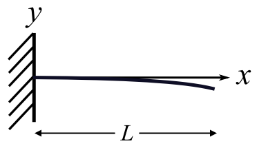
![\[\textcircled{2} \frac{\partial y}{\partial x}(0,t) = 0\]](https://engcourses-uofa.ca/wp-content/ql-cache/quicklatex.com-2bb0c708d1aa8a33b7c9b2318b862598_l3.png "Rendered by QuickLaTeX.com")
![\[\textcircled{3} \frac{\partial ^{2} y}{\partial x^{2}}(L,t) = 0\]](https://engcourses-uofa.ca/wp-content/ql-cache/quicklatex.com-d37fa805611747840fcc2e86ed910eed_l3.png "Rendered by QuickLaTeX.com")
![\[\textcircled{4} \frac{\partial ^{3} y}{\partial x^{3}}(L,t) = 0\]](https://engcourses-uofa.ca/wp-content/ql-cache/quicklatex.com-6025fcfb8f2409e04bdd4dde2b80650a_l3.png "Rendered by QuickLaTeX.com")
gives:
gives:
![\[C_1 + C_3 = 0\]](https://engcourses-uofa.ca/wp-content/ql-cache/quicklatex.com-aa61d7dc55b97598e974fabb990dac79_l3.png "Rendered by QuickLaTeX.com")
Therefore:
![\[Y(x) = C_1(\sin \beta x - \sinh \beta x) + C_2(\cos \beta x - \cosh \beta x)\]](https://engcourses-uofa.ca/wp-content/ql-cache/quicklatex.com-17f2a24424687d27007d5504d556bb4d_l3.png "Rendered by QuickLaTeX.com")
Now, use and respectively
![\[C_1(\sin \beta L + \sinh \beta L) + C_2(\cos \beta L + \cosh \beta L) = 0\]](https://engcourses-uofa.ca/wp-content/ql-cache/quicklatex.com-22a4c277df42a28e5546b98d1b38b415_l3.png "Rendered by QuickLaTeX.com")
![\[C_1(\cos \beta L + \cosh \beta L) - C_2(\sin \beta L - \sinh \beta L) = 0\]](https://engcourses-uofa.ca/wp-content/ql-cache/quicklatex.com-bb92f0a44fc2c001249a4f866db7892b_l3.png "Rendered by QuickLaTeX.com")
For a non-trivial solution the determinant of the coefficients is 0, therefore:
![\[\cos \beta _{r} L \cosh \beta _{r} L = -1\]](https://engcourses-uofa.ca/wp-content/ql-cache/quicklatex.com-0d59541792298666feb929dfa71044d5_l3.png "Rendered by QuickLaTeX.com")
This is a transcendental equation for the  which contains the natural frequencies. In general we can get:
![\[C_2 = \frac{-(\sin \beta _{r} L + \sinh \beta _{r} L)}{(\cos \beta _{r} L + \cosh \beta _{r} L)} C_1\]](https://engcourses-uofa.ca/wp-content/ql-cache/quicklatex.com-be2fd93293fd232d1649d756d36c07a3_l3.png "Rendered by QuickLaTeX.com")
or
![\[C_2 = \frac{(\cos \beta _{r} L + \cosh \beta _{r} L)}{(\sin \beta _{r} L - \sinh \beta _{r} L)} C_1\]](https://engcourses-uofa.ca/wp-content/ql-cache/quicklatex.com-498dd04682b06c9cd98db0441041bde9_l3.png "Rendered by QuickLaTeX.com")
but these are equivalent, therefore the mode shapes are:
![\[Y_{r}(x) = C_1 \bigg[(\sin \beta _{r} x - \sinh \beta _{r} x) + \frac{(\cos \beta _{r} L + \cosh \beta _{r} L)}{(\sin \beta _{r} L - \sinh \beta _{r} L)}(\cos \beta _{r} x - \cosh \beta _{r} x)\bigg]\]](https://engcourses-uofa.ca/wp-content/ql-cache/quicklatex.com-f21b696caca6c6149aadf8f7555e7048_l3.png "Rendered by QuickLaTeX.com")
which is very complicated
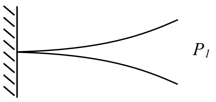
![\[p_1 = (1.875)^{2} \sqrt{\frac{EI}{mL^{4}}}\]](https://engcourses-uofa.ca/wp-content/ql-cache/quicklatex.com-a390dd901ff0976067df5e97254eae5f_l3.png "Rendered by QuickLaTeX.com")
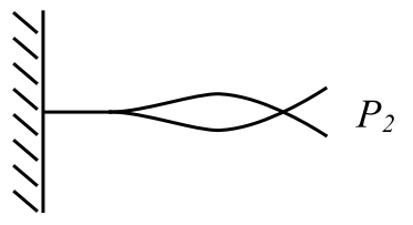
![\[p_2 = (4.694)^{2} \sqrt{\frac{EI}{mL^{4}}}\]](https://engcourses-uofa.ca/wp-content/ql-cache/quicklatex.com-23c4d700f53b218307af755452926444_l3.png "Rendered by QuickLaTeX.com")
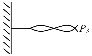
![\[p_3 = (7.855)^{2} \sqrt{\frac{EI}{mL^{4}}}\]](https://engcourses-uofa.ca/wp-content/ql-cache/quicklatex.com-b59155011773fe53549d1f9b87fa0f0b_l3.png "Rendered by QuickLaTeX.com")
This theory works well for the lower frequencies but not for the higher ones since shear and rotation now become important.
we have suggested that these eigenvalues are orthogonal in some sense. While this can be shown in general using operator theory we will show it in a limited way.
Consider two solutions of the general beam vibration problem.
![\[\textcircled{1} \frac{d^{2}}{dx^{2}}\bigg(EI(x)\frac{d^{2}Y_{r}(x)}{dx^{2}}\bigg) = p_{r}^{2} m(x) Y_{r}(x), 0<x<L\]](https://engcourses-uofa.ca/wp-content/ql-cache/quicklatex.com-fe15f0d384294ab36e930d10a23daf3a_l3.png "Rendered by QuickLaTeX.com")
![\[\textcircled{2} \frac{d^{2}}{dx^{2}}\bigg(EI(x)\frac{d^{2}Y_{s}(x)}{dx^{2}}\bigg) = p_{s}^{2} m(x) Y_{s}(x), 0<x<L\]](https://engcourses-uofa.ca/wp-content/ql-cache/quicklatex.com-35d5878bf0f6a25e03e897592ecbad56_l3.png "Rendered by QuickLaTeX.com")
multiply by  and integrate by parts to obtain:
![\[\int _{0}^{L} Y_s(x) \frac{d^{2}}{dx^{2}}\bigg[EI(x)\frac{d^{2}Y_{r}}{dx^{2}}\bigg] dx\]](https://engcourses-uofa.ca/wp-content/ql-cache/quicklatex.com-678e0cc10c2f72b9d777fa3c76e51e93_l3.png "Rendered by QuickLaTeX.com")
![\[\begin{split} &= \bigg[Y_{s}(x) \frac{d}{dx}\bigg\{EI(x)\frac{d^{2}Y_{r}}{dx^{2}}\bigg\}\bigg]_{0}^{L} - \int_{0}^{L} \frac{dY_{s}(x)}{dx} \frac{d}{dx} \bigg\{EI(x)\frac{d^{2}Y_{r}}{dx^{2}}\bigg\} dx \\&= \bigg[Y_{s}(x) \frac{d}{dx}\bigg\{EI(x)\frac{d^{2}Y_{r}}{dx^{2}}\bigg\}\bigg]_{0}^{L} - \bigg[\frac{dY_{s}(x)}{dx} EI \frac{d^{2}Y_{r}}{dx^{2}}\bigg]_{0}^{L} + \int _{0}^{L} EI \frac{d^{2}Y_{s}(x)}{dx^{2}}\frac{d^{2}Y_{r}(x)}{dx^{2}} dx \\&= p_{r}^{2} \int _{0}^{L} m(x) Y_{r}(x) Y_{s}(x) dx \end{split}\]](https://engcourses-uofa.ca/wp-content/ql-cache/quicklatex.com-40485b34d8dee016641fcb025aecdb14_l3.png "Rendered by QuickLaTeX.com")
Now do a similar thing for equation i.e multiply by  and integrate by parts twice. This gives:
![\[\int _{0}^{L} Y_r(x) \frac{d^{2}}{dx^{2}} \bigg\{EI\frac{d^{2}Y_{s}}{dx^{2}}\bigg\} dx\]](https://engcourses-uofa.ca/wp-content/ql-cache/quicklatex.com-b07348dca8c0fc51017c6242cb4688ce_l3.png "Rendered by QuickLaTeX.com")
![\[\begin{split} &= \bigg[Y_r(x) \frac{d}{dx} \bigg\{ EI \frac{d^{2}Y_s}{dx^{2}} \bigg\} \bigg]_{0}^{L} - \bigg[\frac{dY_{r}}{dx} EI \frac{d^{2}Y_s}{dx^{2}} \bigg]_{0}^{L} + \int _{0}^{L} EI \frac{d^{2}Y_r}{dx^{2}}\frac{d^{2}Y_s}{dx^{2}} dx \\&= p_{s}^{2} \int _{0}^{L} m(x) Y_{r}(x) Y_{s}(x) dx \end{split}\]](https://engcourses-uofa.ca/wp-content/ql-cache/quicklatex.com-7f0f50a9e7f4210742b5d743840d6b70_l3.png "Rendered by QuickLaTeX.com")
Subtract these two to give:
![\[(p_r^{2} - p_s^{2}) \int _{0}^{L} m(x) Y_{r}(x) Y_{s}(x) dx = 0 ?\]](https://engcourses-uofa.ca/wp-content/ql-cache/quicklatex.com-195ba893a977ed4ad2591edb0f545da7_l3.png "Rendered by QuickLaTeX.com")
This is clearly true when we have any combination of clamped, simple support, or free ends. It can also be shown to be true when the ends are spring supported.
Therefore, since the eigenvalues are distinct
![\[\int _{0}^{L} m(x) Y_{r}(x) Y_{s}(x) dx = 0\]](https://engcourses-uofa.ca/wp-content/ql-cache/quicklatex.com-271d099814232b2169169d20e3bb2c77_l3.png "Rendered by QuickLaTeX.com")
and they are orthogonal with respect to the mass distribution.
While in the discrete case the eigenvectors were also orthogonal with respect to the stiffness matrix, the eigenfunctions are orthogonal with respect to the stiffness  , only in a certain sense. To see this again consider the eigenvalue problem.
![\[\frac{d^2}{dx^2}\bigg(EI(x) \frac{d^{2}Y_{r}(x)}{dx^{2}}\bigg) = p_{r}^{2}m(x)Y_{r}(x)\]](https://engcourses-uofa.ca/wp-content/ql-cache/quicklatex.com-f7661a531df9e869f33bb3142a7df898_l3.png "Rendered by QuickLaTeX.com")
multiply by  and integrate:
![\[\int _{0}^{L} Y_s(x) \frac{d^{2}}{dx^{2}} \bigg(EI(x)\frac{d^{2}Y_{r}(x)}{dx^{2}}\bigg) = p_{r}^{2} \int m(x)Y_{r}(x) Y_{s}(x) dx\]](https://engcourses-uofa.ca/wp-content/ql-cache/quicklatex.com-4bb117321688e5bc10538b736abe0c42_l3.png "Rendered by QuickLaTeX.com")
But the RHS is zero. Therefore:
![\[\int_0^L Y_s(x)\frac{d^2}{dx^2}\bigg(EI\frac{d^2Y_r(x)}{dx^2}\bigg)dx = 0, \ r\neq s\]](https://engcourses-uofa.ca/wp-content/ql-cache/quicklatex.com-dd4a8f294d29e0711d97814a26236304_l3.png "Rendered by QuickLaTeX.com")
This is somewhat complicated but again we integrate by parts twice to get:
![\[\int_0^L EI(x)\frac{d^2Y_r(x)}{dx^2}\frac{d^2Y_s(x)}{dx^2}dx=0\]](https://engcourses-uofa.ca/wp-content/ql-cache/quicklatex.com-e15465ccf255cefa54431ac889bb889c_l3.png "Rendered by QuickLaTeX.com")
If we use the combination of natural combination of natural and/or geometric b.c.’s.
This says that the second derivative of the eigenfunctions are orthogonal with respect to the stiffness, not the eigenfunctions themselves
When  , we normalize the eigonfunctions as:
![\[\int_0^Lm(x)Y_r(x)Y_s(x)dx = \delta_{rs}\]](https://engcourses-uofa.ca/wp-content/ql-cache/quicklatex.com-3a3ec2b41a44da4af684e9dc4c2fbb7e_l3.png "Rendered by QuickLaTeX.com")
then:
![\[\int Y_s(x)\frac{d^2}{dx^2}\bigg(EI\frac{d^2Y_r(x)}{dx^2}\bigg)dx =p^2_r\delta_{rs}\]](https://engcourses-uofa.ca/wp-content/ql-cache/quicklatex.com-fa8c6615d0547331f8bb4c8510302de6_l3.png "Rendered by QuickLaTeX.com")
If we have one end which has a concentrated mass  then these results must be modified.
For example the corresponding orthogonality becomes:
![\[\int_0^Lm(x)Y_r(x)Y_s(x)dx+MY_r(L)Y_s(L) = 0, \ r\neq s\]](https://engcourses-uofa.ca/wp-content/ql-cache/quicklatex.com-4fe67df97e467185589a1e46527b93a4_l3.png "Rendered by QuickLaTeX.com")
NOTE:
1. The integrals are symmetric with respect to  &
&  . This is similar to the requirement that
  and
and  for discrete systems.
2. Again there could be rigid body modes which means the system is positive semi-definite rather than positive definite. Again we would have to use conservation of linear momentum to exclude these modes.
All this leads to the expansion theorem for continuous systems.
Any function , satisfying the boundary conditions of the problem and such that ![\frac{d^2}{dx^2}\bigg[EI(x)\frac{d^2Y(x)}{dx^2}\bigg]](https://engcourses-uofa.ca/wp-content/ql-cache/quicklatex.com-8fa700fb8b59bd3cd5d145d839dc3db4_l3.png "Rendered by QuickLaTeX.com") is a continuous function can be represented by the absolutely and uniformly convergent series of the system eigenfunctions.
is a continuous function can be represented by the absolutely and uniformly convergent series of the system eigenfunctions.
![\[Y(x) = \sum_{x=1}^\infty C_rY_r(x)\]](https://engcourses-uofa.ca/wp-content/ql-cache/quicklatex.com-55736dbb9b36c38c8c7d72b9db06786c_l3.png "Rendered by QuickLaTeX.com")
where:
![\[C_r = \int_0^Lm(x)Y(x)Y_r(x)dx, \ r = 1,2,...\]](https://engcourses-uofa.ca/wp-content/ql-cache/quicklatex.com-42ccde0621485aae13ffbe5881d205e0_l3.png "Rendered by QuickLaTeX.com")
This is essentially a “generalized” Fourier expansion. In fact when the eigenfunctions are harmonic the expansion theorem does reduce to a Fourier series representation.
Modal Analysis for Continuous Systems
The response of a system to initial excitation external excitation or both can be obtained conveniently by modal analysis. The method is entirely analogous to that for discrete systems which means we must first find the eigenvalues and eigenfunctions. This is of course not trivial.
As an illustration, consider a bar with both edges hinged and with initial conditions:
![\[y(x,0) = y_0(x)\]](https://engcourses-uofa.ca/wp-content/ql-cache/quicklatex.com-3d585b20a843e2b720001c4b57d029a6_l3.png "Rendered by QuickLaTeX.com")
![\[\frac{\partial y(x,t)}{\partial t}\bigg|_{t=0} v_0(x)\]](https://engcourses-uofa.ca/wp-content/ql-cache/quicklatex.com-ebfeebb2faa6703fc5e07a09f15c0594_l3.png "Rendered by QuickLaTeX.com")
The original boundary value problem for a uniform bar is:
![\[-EI\frac{\partial^4y}{\partial x^4} +f(x,t) = m\frac{\partial^2y(x,t)}{\partial t^2}, \ 0<x<L\]](https://engcourses-uofa.ca/wp-content/ql-cache/quicklatex.com-92c5d0cd68c1424b2c43294b1fd7f9e0_l3.png "Rendered by QuickLaTeX.com")
![\[y(0,t) = 0, \quad EI\frac{\partial^2y}{\partial x^2}\bigg|_{x = 0} = 0\]](https://engcourses-uofa.ca/wp-content/ql-cache/quicklatex.com-cf1821a68db0fdcbc8f8f4a1eb1f8851_l3.png "Rendered by QuickLaTeX.com")
![\[y(L,t) = 0, \quad EI\frac{\partial^2y}{\partial x^2}\bigg|_{x = L} = 0\]](https://engcourses-uofa.ca/wp-content/ql-cache/quicklatex.com-64028ccfb9ab791c62fba9534fef6c89_l3.png "Rendered by QuickLaTeX.com")
We also know the solution to the eigenvalue problem for natural frequencies and mode shapes is:
![\[p_r = (r\pi)^2\sqrt{\frac{EI}{mL^4}}, \ r = 1,2,...\]](https://engcourses-uofa.ca/wp-content/ql-cache/quicklatex.com-4afe4428ef737ddb9af0e99622ecfe52_l3.png "Rendered by QuickLaTeX.com")
![\[Y_r(x) = \sqrt{\frac{2}{ml}}\sin\frac{r\pi x}{L}\]](https://engcourses-uofa.ca/wp-content/ql-cache/quicklatex.com-a3fe2d0aa6cb54b3b7a8657e3322d283_l3.png "Rendered by QuickLaTeX.com")
We let the solution of the original equation be of the form:
![\[y(x,t) = \sum_{r = 1}^\infty Y_r(x)\eta_r(t) \quad (\star)\]](https://engcourses-uofa.ca/wp-content/ql-cache/quicklatex.com-2738eb76181c3f11a2014944a96bac53_l3.png "Rendered by QuickLaTeX.com")
This is analogous to the situation in discrete systems in which we used the modal matrix ![[\mu]](https://engcourses-uofa.ca/wp-content/ql-cache/quicklatex.com-9c5362d384456e76e359ae6e37e63a7a_l3.png "Rendered by QuickLaTeX.com") to transform the vector of coordinates
to transform the vector of coordinates  into the normal coordinates
 ![[\eta(t)]](https://engcourses-uofa.ca/wp-content/ql-cache/quicklatex.com-c5a407bccbdf575a2233f285c147d010_l3.png "Rendered by QuickLaTeX.com") . Here instead of the matrix we use the eigenfunctions of the problem.
. Here instead of the matrix we use the eigenfunctions of the problem.
If we put  into:
into:
![\[-EI\frac{\partial^4y}{\partial x^2} + f(x,t) = m\frac{\partial^2y}{\partial t^2}\]](https://engcourses-uofa.ca/wp-content/ql-cache/quicklatex.com-d673c4b5b84e9cb2c467df03c31dd64b_l3.png "Rendered by QuickLaTeX.com")
we get:
![\[\sum_{r=1}^\infty \ddot\eta_r(t)Y_r(x) + \sum_{r=1}^\infty\eta_r(t)EI\frac{d^4Y_r(x)}{dx^4} = f(x, t)\]](https://engcourses-uofa.ca/wp-content/ql-cache/quicklatex.com-c603b7f836043a92ade4707d88de6634_l3.png "Rendered by QuickLaTeX.com")
Multiply by and integrate with respect to to get:
![\[\ddot\eta_r(t) + p^2_r\eta_r(t) = Q_r(t)\]](https://engcourses-uofa.ca/wp-content/ql-cache/quicklatex.com-61c8bd5ca2d43567ad96d95c8956585f_l3.png "Rendered by QuickLaTeX.com")
Where  are the generalized forces associated with the normal coordinates
  . The resulting differential equation is again a SDOF system and its general solution is:
![\[\eta_r(t) = \frac{1}{p_r}\int Q_r(\tau)\sin p_r(t-\tau)d\tau + \eta_{r0}\cos p_rt + \frac{\dot\eta_{r0}}{p_r}\sin p_rt\]](https://engcourses-uofa.ca/wp-content/ql-cache/quicklatex.com-dfd2122e6c899f2f049ce2e6728ed2fe_l3.png "Rendered by QuickLaTeX.com")
where  , where again:
![\[\eta_{r0} = \int_0^Lmy_0(x)Y_r(x)dx,\ r = 1,2,...\]](https://engcourses-uofa.ca/wp-content/ql-cache/quicklatex.com-4602f419e90ad26313388edd1e256b0b_l3.png "Rendered by QuickLaTeX.com")
![\[\dot\eta_{r0} = \int_0^Lm\dot y_0(x)Y_r(x)dx,\ r = 1,2,…\]](https://engcourses-uofa.ca/wp-content/ql-cache/quicklatex.com-5296b75526d27c39d6b3f983c817799e_l3.png "Rendered by QuickLaTeX.com")
The general response is obtained by inserting back into .
Example
![\[f(x,t) = F_0H(t)\]](https://engcourses-uofa.ca/wp-content/ql-cache/quicklatex.com-7754233332412b0020c545feff8c33f0_l3.png "Rendered by QuickLaTeX.com")
![\[y(x,0) = 0, \ \dot y(x,0) = 0\]](https://engcourses-uofa.ca/wp-content/ql-cache/quicklatex.com-78f7bc939fbe7d5182e376748297122a_l3.png "Rendered by QuickLaTeX.com")
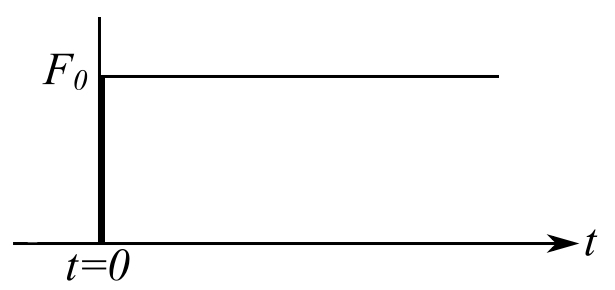
![\[ \begin{split}Q_r(t) &= \int_0^LF_0Y_r(x)dx \\&= F_0H(t)\sqrt{\frac{2}{mL}}\int_0^L\sin\frac{r\pi x}{L} dx \\&= F_0H(t)\sqrt{\frac{2}{mL}}(1-\cos r\pi)\frac{L}{\pi r}, \ r = 1,2,3\\&= \frac{2LF_0H(t)}{\pi r}\sqrt{\frac{2}{mL}}, \ r = 1,3,5 \end{split}\]](https://engcourses-uofa.ca/wp-content/ql-cache/quicklatex.com-4aa6535c0538f4fe2cc4a12ada16d067_l3.png "Rendered by QuickLaTeX.com")
Therefore only odd modes excited by uniform load.
![\[\begin{split}\eta_r &= \frac{1}{p_r}2\sqrt{\frac{2}{mL}}\left(\frac{LF_0}{\pi r}\right)\int_0^t\sin p_r(t-\tau)d\tau \\&= \frac{1}{p_r}2\sqrt{\frac{2}{mL}}\left(\frac{LF_0}{\pi r}\right)\frac{\cos p_r(t-\tau)}{p_r}\bigg]_0^t \\&= \frac{1}{p_r}2\sqrt{\frac{2}{mL}}\left(\frac{LF_0}{\pi r}\right)\bigg[1-\cos p_r t\bigg]\end{split}\]](https://engcourses-uofa.ca/wp-content/ql-cache/quicklatex.com-15cd058904ab0bb5af94710a863927c4_l3.png "Rendered by QuickLaTeX.com")
Therefore:
![\[ y(x,t) = \frac{4F_0L^4}{\pi^5EI}\sum_{r = 1}^\infty \frac{1}{(2r-1)^5}\sin\frac{(2r-1)\pi x}{L}\bigg[1-\cos(2r-1)^2\pi^2\sqrt{\frac{EI}{mL^4}}t\bigg] \]](https://engcourses-uofa.ca/wp-content/ql-cache/quicklatex.com-ef5d7f98b6cae6d02b6c942ef6df0e49_l3.png "Rendered by QuickLaTeX.com")
(NOTE:  now).
now).
It is easy to see that the first mode is predominant.
1st Term:
![\[y_1 = \frac{4F_0L^4}{\pi^5EI}\frac{1}{1^5}\sin\frac{\pi x}{L}\bigg[ 1 - \cos\pi^2\sqrt{\frac{EI}{mL^4}}t\bigg]\]](https://engcourses-uofa.ca/wp-content/ql-cache/quicklatex.com-4cd0c0901d770fbf4db4881aa5466279_l3.png "Rendered by QuickLaTeX.com")
![\[y_{1\text{(MAX)}} = \frac{4F_0L^4}{\pi^5EI}(2) \]](https://engcourses-uofa.ca/wp-content/ql-cache/quicklatex.com-cd6909bd7ce6070bb749f076ff0502d2_l3.png "Rendered by QuickLaTeX.com")
![\[\begin{split}y_{2\text{(MAX)}} &= \frac{4F_0L^4}{\pi^5EI}\bigg(\frac{1}{3^5}\bigg)(2) \\&= 0.004y_{1\text{(MAX)}}\end{split}\]](https://engcourses-uofa.ca/wp-content/ql-cache/quicklatex.com-859032baf044b94550b88dca73d4e6d7_l3.png "Rendered by QuickLaTeX.com")
![\[y_{\text{STATIC(MAX)}} = \frac{5}{384}\frac{F_0L^4}{EI}\]](https://engcourses-uofa.ca/wp-content/ql-cache/quicklatex.com-b0a28298c6ab0dbd0cc9ce0bf03b7892_l3.png "Rendered by QuickLaTeX.com")
![\[\frac{y_{\text{DYNAMIC}}}{y_{\text{STATIC}}}\bigg|_{\text{MAX}} = \frac{2\cdot 4}{\pi^5}\left(\frac{384}{5}\right) =\underline{\underline{2.01}}\]](https://engcourses-uofa.ca/wp-content/ql-cache/quicklatex.com-a3090f64ce4fbc08fd8355e0918d06be_l3.png "Rendered by QuickLaTeX.com")
Effect of Axial Force
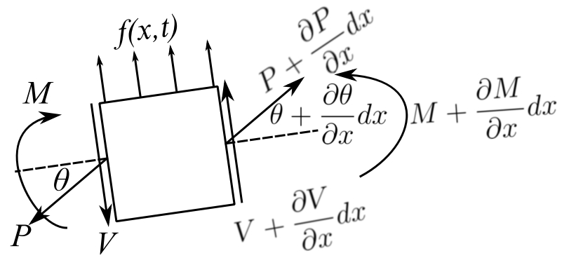
![\[\theta = \frac{\partial y}{\partial x}\]](https://engcourses-uofa.ca/wp-content/ql-cache/quicklatex.com-b0310c009a85714931be76b2db831df6_l3.png "Rendered by QuickLaTeX.com")
![\[\bigg(V+\frac{\partial V}{\partial x}dx\bigg) - V + f(x,t)dx + p+\frac{\partial p}{\partial x}dx\bigg(\frac{\partial y}{\partial x} +\frac{\partial^2 y}{\partial x^2}dx\bigg) - p\frac{\partial y}{\partial x} = mdx\frac{\partial^2 y}{\partial x^2}\]](https://engcourses-uofa.ca/wp-content/ql-cache/quicklatex.com-143a1a36d484ebe3a2aa9a186e2d551d_l3.png "Rendered by QuickLaTeX.com")
From the moment equation:
![\[\frac{\partial M}{\partial x} = -V\]](https://engcourses-uofa.ca/wp-content/ql-cache/quicklatex.com-c8ac723f972e3fe43f8b28498fa02959_l3.png "Rendered by QuickLaTeX.com")
![\[\theta = \frac{\partial y}{\partial x} \]](https://engcourses-uofa.ca/wp-content/ql-cache/quicklatex.com-69d206451f839bd02b843b2f3672d247_l3.png "Rendered by QuickLaTeX.com")
![\[ \theta + N\theta = \frac{\partial y}{\partial x} + \frac{\partial^2y}{\partial x^2}dx\]](https://engcourses-uofa.ca/wp-content/ql-cache/quicklatex.com-dcc10d2a572a726f0d9670d961c714d7_l3.png "Rendered by QuickLaTeX.com")
![\[M = EI\frac{\partial^2y}{\partial x^2}\]](https://engcourses-uofa.ca/wp-content/ql-cache/quicklatex.com-eea95dcdaceedd49ff3f328cc87da91f_l3.png "Rendered by QuickLaTeX.com")
![\[\frac{\partial^2}{\partial x^2}\bigg( EI(x)\frac{\partial^2 y}{\partial x^2}\bigg) + m\frac{\partial^2 y}{\partial t^2} - p\frac{\partial^2y}{\partial x^2} = f(x,t)\]](https://engcourses-uofa.ca/wp-content/ql-cache/quicklatex.com-5023a659a16951db7f70b0261a80020e_l3.png "Rendered by QuickLaTeX.com")
Therefore:
Again we look for the eigenvalues and eigenfunctions by looking at a variables separable solution.
![\[ y(x,t) = Y(x)G(t)\]](https://engcourses-uofa.ca/wp-content/ql-cache/quicklatex.com-74176150d548261fbce86076d00faa37_l3.png "Rendered by QuickLaTeX.com")
Therefore:
![\[y(x,t) = Y(x)\cos(pt - \phi)\]](https://engcourses-uofa.ca/wp-content/ql-cache/quicklatex.com-e0e4b7c680bf7320ccc83e1f1ced0f6e_l3.png "Rendered by QuickLaTeX.com")
And for uniform beams:
![\[IE\frac{d^4Y}{dx^4} - mp^2Y(x) - p\frac{d^2Y}{dx^2} = 0\]](https://engcourses-uofa.ca/wp-content/ql-cache/quicklatex.com-ed312847f86f9ab8d4ab55a0f7a3f505_l3.png "Rendered by QuickLaTeX.com")
![\[Y(x) = e^{sx}\]](https://engcourses-uofa.ca/wp-content/ql-cache/quicklatex.com-9eaff20941236fcb25c9cc28b7c2a493_l3.png "Rendered by QuickLaTeX.com")
![\[s^4 - \frac{p}{EI}s^2 - \frac{mp^2}{EI} = 0\]](https://engcourses-uofa.ca/wp-content/ql-cache/quicklatex.com-f2ebc04c02e8e35e0230e0e596659cd0_l3.png "Rendered by QuickLaTeX.com")
![\[s^2 = \frac{p}{2EI}\pm\sqrt{\frac{p^2}{4E^2I^2}+ \frac{mp^2}{EI}}\]](https://engcourses-uofa.ca/wp-content/ql-cache/quicklatex.com-96661a8095a19ebcfe7f4feaa64f40f1_l3.png "Rendered by QuickLaTeX.com")
Therefore:
![\[S^2_1 = \frac{p}{2EI} + \sqrt{\frac{p^2}{4R^2I^2} + \frac{mp^2}{EI}} = \delta^2 \ \text{(positive)}\]](https://engcourses-uofa.ca/wp-content/ql-cache/quicklatex.com-ce756c62df9141af1295f0e3302c4793_l3.png "Rendered by QuickLaTeX.com")
![\[S^2_2 = \frac{p}{2EI} + \sqrt{\frac{p^2}{4R^2I^2} - \frac{mp^2}{EI}} = -\gamma^2 \ \text{(negative)}\]](https://engcourses-uofa.ca/wp-content/ql-cache/quicklatex.com-2554fe1c5a8b72edce9563a542a0588a_l3.png "Rendered by QuickLaTeX.com")
Therefore:
![\[ S_1 = -\delta^2, \quad S_2 = \pm i\gamma\]](https://engcourses-uofa.ca/wp-content/ql-cache/quicklatex.com-5739e8652636b0845c386953100834cc_l3.png "Rendered by QuickLaTeX.com")
Therefore:
![\[Y(x) = C_1\cosh \delta x + C_2\sinh \delta x + C_3\cos\gamma x + C_4\sin \gamma x \]](https://engcourses-uofa.ca/wp-content/ql-cache/quicklatex.com-585192917e0f18cf25c219d1413219af_l3.png "Rendered by QuickLaTeX.com")
For the S.S case:
![\[Y(0) = Y(L) = 0, \ Y''(0) = Y''(L) = 0\]](https://engcourses-uofa.ca/wp-content/ql-cache/quicklatex.com-30ee8ee748bb546db24aa4b35c91c5b5_l3.png "Rendered by QuickLaTeX.com")
![\[C_1 +C_3 = 0, \ C_1\delta^2 - C_3\gamma^ 2 = 0, \ C_3 = -C_1\]](https://engcourses-uofa.ca/wp-content/ql-cache/quicklatex.com-777466d293511fb4d15d9a6bf93e28ff_l3.png "Rendered by QuickLaTeX.com")
Therefore:
![\[C_1(\delta^2 +\gamma^2) = 0\]](https://engcourses-uofa.ca/wp-content/ql-cache/quicklatex.com-188377bd9ec0a496aad43de6ee63441a_l3.png "Rendered by QuickLaTeX.com")
Therefore:
![\[C_1\bigg[ \frac{p}{2EI} + \sqrt{\frac{p^4}{4E^2I^2} + \frac{mp^2}{EI}} - \frac{p}{2EI} + \sqrt{\frac{p^4}{4E^2I^2} + \frac{mp^2}{EI}}\bigg] = 2C_1\sqrt{\frac{p^4}{4E^2I^2} + \frac{mp^2}{EI}} = 0\]](https://engcourses-uofa.ca/wp-content/ql-cache/quicklatex.com-0092f472de5835ab68495622e91e842f_l3.png "Rendered by QuickLaTeX.com")
Therefore:
![\[C_1 = 0, \ C_3 = 0\]](https://engcourses-uofa.ca/wp-content/ql-cache/quicklatex.com-88d3d955fb13a8b9ceff762c7c16adb9_l3.png "Rendered by QuickLaTeX.com")
![\[Y(L) = C_2\sinh\delta L + C_4\sin \gamma L = 0\]](https://engcourses-uofa.ca/wp-content/ql-cache/quicklatex.com-4e34066deece6028a90eba6da7aa268d_l3.png "Rendered by QuickLaTeX.com")
![\[Y''(L) = C_2\delta^2\sinh\delta L - C_4\gamma^2\sin\gamma L = 0\]](https://engcourses-uofa.ca/wp-content/ql-cache/quicklatex.com-bea5dd7624553b94948cf32b5690bc14_l3.png "Rendered by QuickLaTeX.com")
Multiply by  and add to get:
![\[C_2(\gamma^2 + \delta^2)\sinh\delta L = 0\]](https://engcourses-uofa.ca/wp-content/ql-cache/quicklatex.com-f7ed237a0c2e93ab4f61f279e3deeb1d_l3.png "Rendered by QuickLaTeX.com")
![\[ \implies C_2 = 0\]](https://engcourses-uofa.ca/wp-content/ql-cache/quicklatex.com-25f72816f60f57ae6e984cabe31de388_l3.png "Rendered by QuickLaTeX.com")
Therefore:
![\[\sin\gamma L = 0\]](https://engcourses-uofa.ca/wp-content/ql-cache/quicklatex.com-2af0ab30fa65dc4734e00b5499fc21e3_l3.png "Rendered by QuickLaTeX.com")
![\[ \gamma L = r\pi, \quad r = 1,2,3...\]](https://engcourses-uofa.ca/wp-content/ql-cache/quicklatex.com-b0238f9f3bf2f1565625277180f1eef2_l3.png "Rendered by QuickLaTeX.com")
![\[ \gamma^2 = \bigg(\frac{r\pi}{L}\bigg)^2 = -\frac{p}{2EI} + \sqrt{\frac{p^2}{4E^2I^2} + \frac{mp^2}{EI}}\]](https://engcourses-uofa.ca/wp-content/ql-cache/quicklatex.com-0ed212cc46b7af362f3faa14b13293ec_l3.png "Rendered by QuickLaTeX.com")
![\[\frac{p}{2EI} + \bigg(\frac{r\pi}{L}\bigg)^2 = \sqrt{\frac{p^2}{4E^2I^2} + \frac{mp^2}{EI}}\]](https://engcourses-uofa.ca/wp-content/ql-cache/quicklatex.com-e12a2f0b1d1c565841d783842eb34507_l3.png "Rendered by QuickLaTeX.com")
![\[\frac{p^2}{4E^2I^2} + \frac{2p}{2EI}\bigg(\frac{r\pi}{L}\bigg)^2 + \frac{r^4\pi^4}{L^4} = \frac{p^2}{4E^2I^2} + \frac{mp^2}{EI}\]](https://engcourses-uofa.ca/wp-content/ql-cache/quicklatex.com-14d506e20f5d20cffdf900adbcbb148e_l3.png "Rendered by QuickLaTeX.com")
Therefore :
![\[\begin{split}p^2 &= \frac{EI}{m}\bigg[\frac{r^4\pi^2}{L^4} +\frac{r^2\pi^2}{L^4}\frac{p}{EI}\bigg] \\&= \frac{EI\pi^4}{mL^4}\bigg[ r^4 + \frac{r^2pl^2}{\pi^2EI}\bigg]\end{split}\]](https://engcourses-uofa.ca/wp-content/ql-cache/quicklatex.com-cf10f7ca55d880df4591a3d682b963c9_l3.png "Rendered by QuickLaTeX.com")
![\[p = \pi^2\sqrt{\frac{EI}{ml^4}}\bigg[r^4 + \frac{r^2pL^2}{\pi^2EI}\bigg] ^{\frac{1}{2}}\]](https://engcourses-uofa.ca/wp-content/ql-cache/quicklatex.com-0e0d453c601ee596c191fbc2cc8eb29b_l3.png "Rendered by QuickLaTeX.com")
Special Cases:
- if
 :
:![\[ p = r^2\pi^2\sqrt{\frac{EI}{ml^4}} \ \text{(S.S beam as before)}\]](https://engcourses-uofa.ca/wp-content/ql-cache/quicklatex.com-29b79eac9e35781877c717ffe895ae6f_l3.png "Rendered by QuickLaTeX.com")
- if
 :
:![\[ p = \pi^2\sqrt{\frac{EI}{ml^4}}\frac{r}{\pi}\sqrt{\frac{pL^2}{EI}}\]](https://engcourses-uofa.ca/wp-content/ql-cache/quicklatex.com-d93fc244a5ac39c7ff0d32b7fd2e9e4a_l3.png "Rendered by QuickLaTeX.com")
![\[p = \frac{r\pi}{L}\sqrt{\frac{p}{m}} = \frac{r\pi}{L}\sqrt{\frac{p}{\rho}} \ \text{(string result)}\]](https://engcourses-uofa.ca/wp-content/ql-cache/quicklatex.com-8f2bae2876e9ae432c3118716efb604d_l3.png "Rendered by QuickLaTeX.com")
 , then the natural frequencies are higher than without axial force.
 , then the natural frequencies decrease from that without axial force.
as ,
,  .
.
This is the state buckling load of the beam. The effect of axial load can be used as a technique to estimate the load in a particular member.
Approximate Methods for Beams
It is obvious that only a few problems can be solved analytically for beam vibrations. As a result, approximate methods, including FEA, are necessary. There are a few approximate methods that can be used to give a crude approximation and require relatively little work.
We well consider the Rayleigh’s Quotient and from it Dunkerley’s Method. These allow bounding of the lowest natural frequency and can be used as a starting point for more sophisticated techniques. They are based on an energy approach similar to that used for finite dimensional problems.
Rayleigh’s Quotient
Again we find the kinetic and potential energy assuming SSHM for the particles of a beam.
The kinetic energy of  is
is
![\[ \frac{1}{2}mdx\Big(\frac{\partial y}{\partial t}\Big)^2 \]](https://engcourses-uofa.ca/wp-content/ql-cache/quicklatex.com-95ddb71fad3ce453afd0e165373a5757_l3.png "Rendered by QuickLaTeX.com")
Therefore the total kinetic energy of the beam is
![\[ T = \int_L \frac{1}{2}m\Big(\frac{\partial y}{\partial t}\Big)^2dx \]](https://engcourses-uofa.ca/wp-content/ql-cache/quicklatex.com-3149f730a84a10c31da9f7ae58cf872b_l3.png "Rendered by QuickLaTeX.com")
where we integrate over the entire beam.
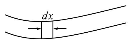
To find the potential energy (stored in the beam) consider the bending of an element from its static shape.

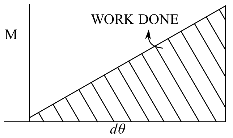
The work done is 
![\[ \theta \approx \frac{\partial y}{\partial x} \]](https://engcourses-uofa.ca/wp-content/ql-cache/quicklatex.com-f114d29f93fc600e855aa8fbfebe79d9_l3.png "Rendered by QuickLaTeX.com")
Therefore:
![\[ d\theta = \frac{\partial^2y}{\partial x^2}dx \]](https://engcourses-uofa.ca/wp-content/ql-cache/quicklatex.com-223919309e5cbc64404a47e7cffaeb1a_l3.png "Rendered by QuickLaTeX.com")
![\[ M = EI \frac{\partial^2y}{\partial x^2} \qquad \text{(as before)} \]](https://engcourses-uofa.ca/wp-content/ql-cache/quicklatex.com-4e0fef040855a880984829452cf520ed_l3.png "Rendered by QuickLaTeX.com")
Therefore work done on the element
![\[ = \frac{1}{2}EI\Big(\frac{\partial^2 y}{\partial x^2}\Big)^2dx \]](https://engcourses-uofa.ca/wp-content/ql-cache/quicklatex.com-00d513ea66f6a6e577f47701b9edc0f1_l3.png "Rendered by QuickLaTeX.com")
and the energy stored is the total work done on the entire beam
![\[ U = \int_L \frac{1}{2}EI\Big(\frac{\partial^2 y}{\partial x^2}\Big)^2dx \]](https://engcourses-uofa.ca/wp-content/ql-cache/quicklatex.com-da1db12d49d02c0db587888792ec8769_l3.png "Rendered by QuickLaTeX.com")
Rayleigh again assume SSHM and 
Therefore assume 
![\[ \begin{split} \frac{\partial^2y}{\partial x^2} &= \frac{d^2Y}{dx^2}\sin(pt+\phi) \\ \frac{\partial y}{\partial t} &= -Y(x)\cos(pt+\phi) \end{split} \]](https://engcourses-uofa.ca/wp-content/ql-cache/quicklatex.com-28cdbd0926a04220a820d4a2ec003f93_l3.png "Rendered by QuickLaTeX.com")
![\[ \begin{split} U_{\text{MAX}} &= V_{\text{MAX}} \\ U_{\text{MAX}} &= \frac{1}{2}\int_0^L EI \Big(\frac{d^2Y}{dx^2}\Big)^2dx \\ V_{\text{MAX}} &= \frac{1}{2}p^2\int_0^L m(Y)^2dx \\ p^2 &= \frac{\int_0^L EI \Big(\frac{d^2Y}{dx^2}\Big)^2dx}{\int_0^L m(Y)^2dx} \end{split} \]](https://engcourses-uofa.ca/wp-content/ql-cache/quicklatex.com-128d8271ef2607042d7183bc5f1e96c5_l3.png "Rendered by QuickLaTeX.com")
but we must have the exact mode shape to get the right answer. It can be shown that we can get an upper bound for  if we select a shape function (mode shape) which satisfies the geometric b.c.
![\[ p^2 \leq \frac{\int_L EI \big(\frac{d^2Y}{dx^2}\big)^2dx}{\int_L m \{Y\}^2dx} \]](https://engcourses-uofa.ca/wp-content/ql-cache/quicklatex.com-0d81888aa6b912fd11b9e9c186620b69_l3.png "Rendered by QuickLaTeX.com")
e.g. Cantilever Beam
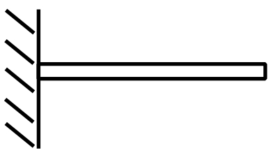
![\[ \begin{split} Y(x) &= Ax^2 \\ Y'(x) &= 2Ax \\ Y''(x) &= 2A \end{split} \]](https://engcourses-uofa.ca/wp-content/ql-cache/quicklatex.com-155292e4fc0674d0b67c1eeadeb8963e_l3.png "Rendered by QuickLaTeX.com")
![\[ \begin{split} p_1^2 \leq \frac{\int_0^L EI(4A)^2dx}{\int_0^L mA^2x^4dx} &= \frac{4EIL}{mx^5/5\big]_0^L} \\ &= \frac{20EI}{mL^4} \end{split} \]](https://engcourses-uofa.ca/wp-content/ql-cache/quicklatex.com-5169ffdc2cd2bafb2c55bc27e3794984_l3.png "Rendered by QuickLaTeX.com")
Therefore:
![\[ \begin{split} p \leq \sqrt{20} \sqrt{\frac{EI}{mL^4}} &= 4.47 \sqrt{\frac{EI}{mL^4}} \\ p_{\text{EXACT}} &= 3.52 \sqrt{\frac{EI}{mL^4}} \end{split} \]](https://engcourses-uofa.ca/wp-content/ql-cache/quicklatex.com-8fc51f21e0220997a929bf6b2c0fecee_l3.png "Rendered by QuickLaTeX.com")
![\[ \begin{split} Y &= Ax^3 \\ Y' &= 3Ax^2 \\ Y'' &= 6Ax \end{split} \]](https://engcourses-uofa.ca/wp-content/ql-cache/quicklatex.com-1271f7bb3c6de46ccc07f77389f3a613_l3.png "Rendered by QuickLaTeX.com")
![\[ \begin{split} p_1^2 \leq \frac{EI\int_0^L 36x^2 dx}{m\int_0^L x^6dx} &= \frac{EI 12L^3}{m L^7/7} \\ p_1^2 \leq \frac{84EI}{mL^4} \\qquad \text{Worse} \end{split} \]](https://engcourses-uofa.ca/wp-content/ql-cache/quicklatex.com-37ffa1c25f8dab30bc96555ea39829b2_l3.png "Rendered by QuickLaTeX.com")
We can extend the idea of Rayleigh to the case in which there are point masses and springs attached at a point on a beam.
Consider first a point mass,  at position
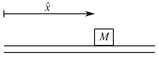
It has kinetic energy T where
![\[ \begin{split} T &= \frac{1}{2}m\Big(\frac{\partial y}{\partial t}\Big|_{x=\hat{x}}\Big)^2 \\ T_{\text{MAX}} &= \frac{1}{2}mp^2\{Y(\hat{x}\}^2 \end{split} \]](https://engcourses-uofa.ca/wp-content/ql-cache/quicklatex.com-b20232c8a08413f122abe359419d594d_l3.png "Rendered by QuickLaTeX.com")
when we assume
![\[ y(x,t,) = Y(x)\sin(pt+\phi) \]](https://engcourses-uofa.ca/wp-content/ql-cache/quicklatex.com-4180fbe106f75388f920508c022d5d00_l3.png "Rendered by QuickLaTeX.com")
For a spring at position 
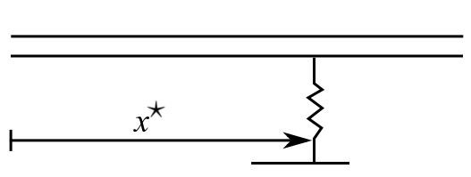
The potential energy 
Again if we assume 
![\[U_{\text{MAX}} = \frac{1}{2}k\{Y(x^*)\}^2 \]](https://engcourses-uofa.ca/wp-content/ql-cache/quicklatex.com-82fe3b430f71dde04ed3222a6b0d77d1_l3.png "Rendered by QuickLaTeX.com")
We simply add these energies to the  and
and  of the beam to get
![\[ p_1^2 \leq \frac{\int_L EI\big(\frac{d^2Y}{dx^2}\big)^2dx + \sum_{i=1}^n k_i{Y(x_i)}^2}{\int_L m{Y(x)}^2dx + \sum^m_{j=1} M_j {Y(x_j)}^2} \]](https://engcourses-uofa.ca/wp-content/ql-cache/quicklatex.com-153c299b6f504d69d7d515bf2a9be8e7_l3.png "Rendered by QuickLaTeX.com")
for  springs and masses
Therefore the integrations are over the entire length of the beam.
We can consider beams width varying X section and varying mass distribution.
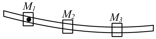
Dunkerley’s Method for Beams is an extension of Rayleigh’s Quotient where there are no additional springs.
Consider a beam carrying several masses
The Rayleigh Quotient is
![\[ p_1^2 = \frac{\int_L EI\big(\frac{d^2Y}{dx^2}\big)^2dx}{\int_L m\{Y\}dx + \sum_{i=1}^r M_i \{Y^*(x_i)\}^2} \]](https://engcourses-uofa.ca/wp-content/ql-cache/quicklatex.com-3b17c98156d9d34c3b1515dea9199b71_l3.png "Rendered by QuickLaTeX.com")
Assume that  is the actual shape function for the combined system so that p_1^2 is the actual natural frequency.
Therefore:
![\[ \frac{1}{p_1^2} = \frac{\int_L m(Y^*)^2 dx}{\int_L EI\big(\frac{d^2Y^*}{dx^2}\big)^2dx} + \frac{\sum^r_{i=1}M_i\{Y^*(x_i)\}^2}{\int_L EI\big(\frac{d^2Y^*}{dx^2}\big)^2dx} \]](https://engcourses-uofa.ca/wp-content/ql-cache/quicklatex.com-3313beea64f1dcf40039f2bbebc52486_l3.png "Rendered by QuickLaTeX.com")
The first term is an approximation to the fundamental frequency of the beam alone
Therefore
![\[ p^2_{1(B)} \leq \frac{\int_L EI\Big(\frac{d^2Y^*}{dx^2}\Big)^2dx}{\int_L m\{Y^*\}^2dx} \]](https://engcourses-uofa.ca/wp-content/ql-cache/quicklatex.com-32c7dd0492b8ef749a3962e115a2cf23_l3.png "Rendered by QuickLaTeX.com")
![\[ \frac{1}{p^2_{1(B)}} \geq \frac{\int_0^L m{Y^*}^2dx}{\int_0^L EI\Big(\frac{d^2Y^*}{dx^2}\Big)^2dx} \]](https://engcourses-uofa.ca/wp-content/ql-cache/quicklatex.com-fa565109fded1018723f5f3d08966b19_l3.png "Rendered by QuickLaTeX.com")
since  is the exact answer for the combined system.
Similarly to each of the added masses.
![\[ \frac{1}{(p_{1i})^2} \geq \frac{M_i\{Y^*(x)\}^2}{\int_0^L EI\big(\frac{d^2Y^*}{dx^2}\big)^2dx} \]](https://engcourses-uofa.ca/wp-content/ql-cache/quicklatex.com-6060ad90bbd678f95e38dc5f6758cf72_l3.png "Rendered by QuickLaTeX.com")
Therefore:
![\[ \frac{1}{p_1^2} \leq \frac{1}{p_{1(B)}^2} + \sum^r_{i=1}\frac{1}{(p_1i)^2} \]](https://engcourses-uofa.ca/wp-content/ql-cache/quicklatex.com-dc09879e3ba0398ed794ee820aeb27bd_l3.png "Rendered by QuickLaTeX.com")
This allows the calculation of the lower bound for the natural frequency 
Example
S.S beam of the mass/length carrying at midspan
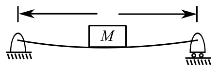
![\[ p^2_{1(B)} = \frac{\pi^4EI}{mL^4} \qquad \qquad \Delta_{L/2} = \frac{M_gL^3}{48EI} \quad (\text{static}) \]](https://engcourses-uofa.ca/wp-content/ql-cache/quicklatex.com-33edc7f321c5a41ed7af53c504f2ed42_l3.png "Rendered by QuickLaTeX.com")
Therefore
![\[ p^2_1 = \frac{g}{\Delta} \]](https://engcourses-uofa.ca/wp-content/ql-cache/quicklatex.com-f8ecf8aed0249bf05dc16671087bb248_l3.png "Rendered by QuickLaTeX.com")
Therefore
![\[ \begin{split} \frac{1}{p_1^2} & \leq \frac{mL^4}{\pi^4EI} + \frac{ML^3}{48EI} \\ &= \frac{48mL^4 + \pi^4ML^3}{48\pi^4EI} \end{split} \]](https://engcourses-uofa.ca/wp-content/ql-cache/quicklatex.com-f402fea058d5da6585929e45f034ab72_l3.png "Rendered by QuickLaTeX.com")
![\[ p_1^2 > \frac{48EI}{L^3\big[M + \frac{48}{\pi^4}mL\big]} = \frac{48EI}{L^3\big[M + 0.493mL\big]} \]](https://engcourses-uofa.ca/wp-content/ql-cache/quicklatex.com-ab37a81318895bfd159a35a494fb5812_l3.png "Rendered by QuickLaTeX.com")
Use Rayleigh to get upper bound. Try:
![\[ \begin{split} Y(x) &= Ax(L-x) \\ &= AxL - Ax^2 \\ Y'(x) &= AL - 2Ax \\ Y''(x) &= -2A \end{split} \]](https://engcourses-uofa.ca/wp-content/ql-cache/quicklatex.com-9e20e005f02d815df29714791b7123b7_l3.png "Rendered by QuickLaTeX.com")
![\[ \begin{split} Y\Big(\frac{L}{2}\Big) &= A\frac{L}{2}\Big(L- \frac{L}{2}\Big) \\ &= \frac{AL^2}{4} \end{split} \]](https://engcourses-uofa.ca/wp-content/ql-cache/quicklatex.com-341420c43d68504f0f062c4c9d1818a6_l3.png "Rendered by QuickLaTeX.com")
![\[ \begin{split} p^2_{1(B)} & \leq \frac{\int^L_0 EI(4A^2)dx}{\int_0^L m(A^2x^2L^2 + A^2x^4 - 2A^2x^3L)dx + M\frac{A^2L^4}{16}} \\ &= \frac{EI4L}{m\big[ \frac{x^3L^2}{3} + \frac{x^5}{5} - \frac{2x^4L}{4} \big]^L_0 + \frac{ML^4}{16}} \\ &= \frac{4EI}{mL^4\big[\frac{1}{3} + \frac{1}{5} - \frac{1}{2}\big] + \frac{ML^3}{16}} \\ &= \frac{4EI}{mL^4 \big[ \frac{10+6-15}{30} \big] + \frac{ML^3}{16}} \\ &= \frac{4EI}{\frac{mL^4}{30} + \frac{ML^3}{16}} \\ &= \frac{48EI}{L^3\big[\frac{3}{4}M + \frac{2}{5}mL\big]} \end{split} \]](https://engcourses-uofa.ca/wp-content/ql-cache/quicklatex.com-99b80d52034422132d577b4b5cb3b74b_l3.png "Rendered by QuickLaTeX.com")
Let 
![\[ \begin{split} p_1^2 &> \frac{48EI}{1.493mL^4} = 32.15 \frac{EI}{mL^4} \\ p_1 &> 5.67\sqrt{\frac{EI}{mL^4}} \end{split} \]](https://engcourses-uofa.ca/wp-content/ql-cache/quicklatex.com-9df90fba8de5381bd6ee5097ef6351f5_l3.png "Rendered by QuickLaTeX.com")
![\[ \begin{split} p_1^2 &< \frac{48EI}{\frac{23}{20}mL^4} = 41.74 \frac{EI}{mL^4} \\ p_1 &< 6.46 \sqrt{\frac{EI}{mL^4}} \end{split} \]](https://engcourses-uofa.ca/wp-content/ql-cache/quicklatex.com-b5b7f6ffe7d8f48183aa5f93c65f56d8_l3.png "Rendered by QuickLaTeX.com")
Vibration of a Free-Free Beam
The bending vibration of a beam are described by the following equation:
![\[ EI \frac{\partial ^4 y}{\partial x^4} + \rho A \frac{\partial ^2 y}{\partial t^2} = 0 \quad (1) \]](https://engcourses-uofa.ca/wp-content/ql-cache/quicklatex.com-89bde503a3804213a6d715e96e4f8c36_l3.png "Rendered by QuickLaTeX.com")
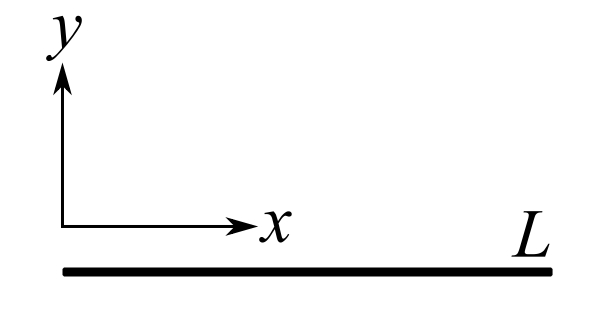
E,I,, A are respectively the Young Modulus, second moment of area of the cross section, density and cross section area of the beam. L is the length of the beam. The solution of Eq.(1) can be written as a standing wave
 , separating the spatial and temporal component. This leads to the following characteristic equation that relates the circular frequency
  to the wavenumber k:
![\[\omega ^2 = \frac{EI}{\rho A}k^4 \quad (2)\]](https://engcourses-uofa.ca/wp-content/ql-cache/quicklatex.com-14c754e6d51266ec495057b3f7790281_l3.png "Rendered by QuickLaTeX.com")
The spatial part can be written as:
![\[w(x) = C_1 \sin(kx) + C_2 \cos(kx) + C_3\sinh(kx) + C_4\cosh(kx) \quad (3)\]](https://engcourses-uofa.ca/wp-content/ql-cache/quicklatex.com-ef5ae31ec7ce7389b05ae2cc81535ed7_l3.png "Rendered by QuickLaTeX.com")
For a Free-Free Beam the boundary conditions are (vanishing of force and moment):

——————————————————————
A standing wave or stationary wave is a wave ‘frozen’ in the space and vibrating in time. It result by the sum of two identical waves travelling in opposite directions:
![\[\begin{split} y(x,t) &= y_+ (x,t) + y_-(x,t) \\&= Y_o \sin (\omega t -kx) + Y_o \sin (\omega t + kx) \\&= 2Y_o \sin (kx) \cos(\omega t) \\&= w(x)u(t) \end{split}\]](https://engcourses-uofa.ca/wp-content/ql-cache/quicklatex.com-2a53ca47b03c32d1eecb22edc61ece07_l3.png "Rendered by QuickLaTeX.com")
Using the first two equations the  and
and  can be arranged in matrix form:

For a non trivial solution the determinant of the matrix has to vanish to get:
![\[\cosh(kL) \cos(kL) = 1 \quad (5)\]](https://engcourses-uofa.ca/wp-content/ql-cache/quicklatex.com-21d01e302b1e86b7ee9a07a135dcf405_l3.png "Rendered by QuickLaTeX.com")
The transcendental Eq.(5) has infinite solutions, it can be solved numerically, the first five values are reported here:
| Mode order n | knL |
| 0 | 0 |
| 1 | 4.7300 |
| 2 | 7.8532 |
| 3 | 10.9956 |
| 4 | 14.1371 |
| 5 | 17.2787 |
Putting these values back in Eq. (5) gives the modeshapes corresponding to the natural frequencies  , that can be calculated from the characteristic Eq. (2). The mode shapes are given by the following:
![\[\omega _n (x) = [\sinh(k_nx) +\sin(k_nx)] + \frac{\sin(k_nL) - \sinh(k_nL)}{\cosh(k_nL) - \cos(k_nL)}[\cosh(k_nx + \cos(k_nx)] \quad (6)\]](https://engcourses-uofa.ca/wp-content/ql-cache/quicklatex.com-a7a9e16f5b27770f164ac8d0f6ebb3dc_l3.png "Rendered by QuickLaTeX.com")
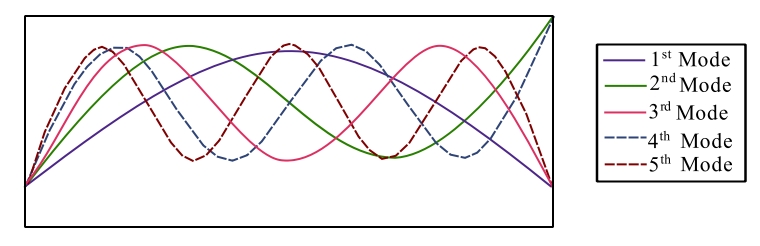
Figure 1: First 5 mode shapes for a free-free beam
While many musical instruments use vibrations as the source of the sound they produce, one of simplest that is very commonly used outdoors is the wind chimes. As illustrated the classical version uses a number (usually 5 or 6) tubes of various lengths and held at various positions that are struck with a central clapper near the center of the tubes. To accomplish this various length tubes are positioned at different lengths relative to the supporting structure. The illustrated chimes are composed of 5 tubes corresponding to a piano’s black keys, making up the so-called minor pentatonic scale. These were first studied by the ancient Greeks (including Pythagoras) who realized the link between the length of a vibrating body and the notes of a musical scale. Actually, the tubes can be treated as free-free beams which are supported at certain positions. A do-it-yourself magazine suggested building your own using 5 copper tubes (3/4 inch type M with an OD = 0.875 in., ID = 0.811 in., weight of 0.328 lbs./ft and Modulus of Elasticity 23 X 10 psi) with:
| Length(in.) | Hang Point (from top) (in.) | Musical pitch |
| 11 1/2 | 2 9/16 | C-sharp |
| 10 7/8 | 2 7/16 | D-sharp |
| 10 | 2 1/4 | F-sharp |
| 9 7/16 | 2 1/8 | G-sharp |
| 8 7/8 | 2 | A-sharp |
a) Calculate the first natural frequency of the five tubes of various lengths
b) Calculate the ratio of the position of the hang point to the total length of each tube. Why is this ratio essentially the same?
c) An 88 key piano keyboard (numbered from 1-88) has standard fundamental frequencies (available on the internet). Find the key numbers that correspond to the 5 tube free-free beam frequencies and show their position on the standard piano keyboard.
How to Make Wind Chimes in 5 Easy Steps
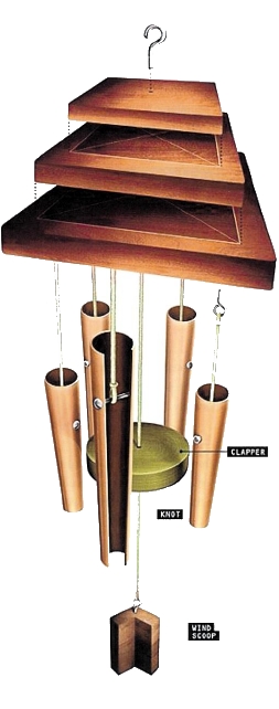
1.) Gather Materials
Round up at least 5 feet of Type M 3/4-inch copper tubing, seven eye screws, five No. 6 1-inch machine screws and nuts, nylon twine, and 1 x 6 lumber.
2.) Map Pipe Mounts
Center a 4 1/2-inch-diameter circle in a 5 1/2-inch-square cut of lumber. Mark the circle at five equidistant points. Insert eye screws at the circle’s center and at all five points.
3.) Cut Pythagoras
Cut five pieces of tubing to the lengths in the table below and deburr. The chime’s five notes, which correspond to a piano’s black keys, make up the minor pentatonic scale. The notes are pleasing in any order. The ancient Greeks such as Pythagoras were the first to study the link between the length of a vibrating body and the notes of a musical scale.
| Musical Pitch | Length 3/4-inch copper | Hang Point from top |
| C-sharp | 11 1/2 inches | 2 9/16 inches |
| D-sharp | 10 7/8 inches | 2 7/16 inches |
| F-sharp | 10 inches | 2 1/4 inches |
| G-sharp | 9 7/16 inches | 2 1/8 inches |
| A-sharp | 8 7/8 inches | 2 inches |
4.) Tie With Twine
Drill a 5/32-inch hole through each pipe as listed in the table. These hanging points produce the best chime resonance. Insert a machine screw through the hole and fit a nut onto the screw shank. Tie a 7-inch length of twine from the circle of eye screws to the screw shank in each pipe.
5.) Hang the Chime
Use a 2 1/2-inch holesaw to cut a clapper from a 1x scrap. Use more 1x waste to make a V-shaped, 3-inch-long wind scoop. Hang each from the center eye screw. Cut and glue two smaller 1x squares to the top of the first square. Top-center-mount an eye screw in the smallest square. Hang the chime in the breeze and enjoy.
Table 1: Dimensions and Physical Characteristics of Copper Tube: TYPE M
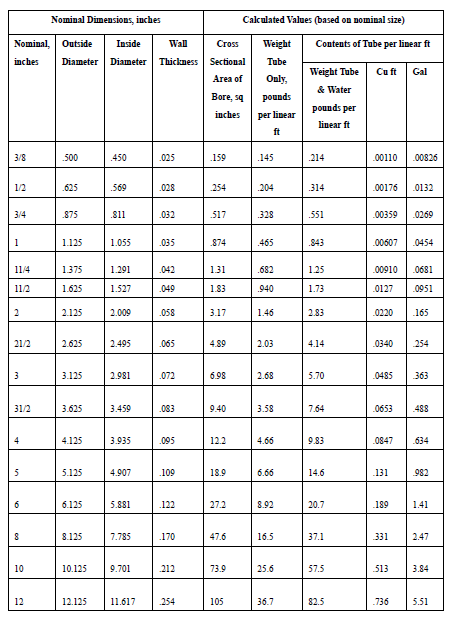
Table 2: Dimensions and Physical Characteristics of Copper Tube: DWV (Drain, Waste and Vent)
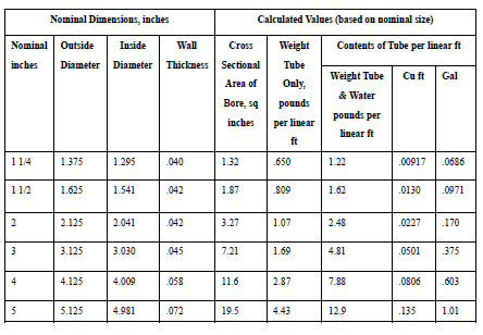
Piano key frequencies
This is a list of the fundamental frequencies in hertz (cycles per second) of the keys of a modern 88-key standard or 108-key extended piano in twelve-tone equal temperament, with the 49th key, the fifth A (called A4), tuned to 440 Hz (referred to as A440). 12 Since every octave is made of twelve steps and equals two times the frequency (for example, the fifth A is 440 Hz and the higher octave A is 880 Hz), each successive pitch is derived by multiplying (ascending) or dividing (descending) the previous by the twelfth root of two (approximately 1.059463). For example, to get the frequency a semitone up from A4 (A#4), multiply 440 by the twelfth root of two. To go from A4 to B4 (up a whole tone, or two semitones), multiply 440 twice by the twelfth root of two (or just by the sixth root of two, approximately 1.122462). To go from A4 to C5 (which is a minor third), multiply 440 three times by the twelfth root of two, (or just by the fourth root of two, approximately 1.189207). For other tuning schemes refer to musical tuning.
This list of frequencies is for a theoretically ideal piano. On an actual piano the ratio between semitones is slightly larger, especially at the high and low ends, where string stiffness causes inharmonicity, i.e., the tendency for the harmonic makeup of each note to run sharp. To compensate for this, octaves are tuned slightly wide, stretched according to the inharmonic characteristics of each instrument. This deviation from equal temperament is called the Railsback curve. The following equation gives the frequency f of the nth key, as shown in the table:
The following equation gives the frequency f of the nth key, as shown in the table:
![\[f(n) = (\sqrt[12]{2})^{n-49} \times 440 \text{Hz}\]](https://engcourses-uofa.ca/wp-content/ql-cache/quicklatex.com-36b2a96397dd1a83ce31f30e0e069a53_l3.png "Rendered by QuickLaTeX.com")
(a’ = A4 = A440 is the 49th key on the idealized standard piano)
Alternatively, this can be written as:
![\[f(n) = 2^{\frac{n-49}{12}} \times 440 \text{Hz}\]](https://engcourses-uofa.ca/wp-content/ql-cache/quicklatex.com-325a5a797b6ddb86aef8ac396b16fe7b_l3.png "Rendered by QuickLaTeX.com")
Conversely, starting from a frequency on the idealized standard piano tuned to A440, one obtains the key number by:
![\[\begin{split} n &= 12 \log_2(\frac{f}{440\text{Hz}}) + 49 \\&= 39.86 \log _{10} (\frac{f}{440\text{Hz}}) + 49 \end{split}\]](https://engcourses-uofa.ca/wp-content/ql-cache/quicklatex.com-4bdbd58f322fe418e181d25816db3eed_l3.png "Rendered by QuickLaTeX.com")
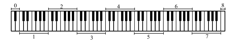
An 88-key piano, with the octaves numbered and Middle C (cyan) and A440 (yellow) highlighted
Values in bold are exact on an ideal piano. Keys shaded gray are rare and only appear on extended pianos. The normally included 88 keys have been numbered 1-88, with the extra low keys numbered 89-97 and the extra high keys numbered 98-108. (A 108-key piano that extends from Co to B8 was first built in 2018 by Stuart & Sons.
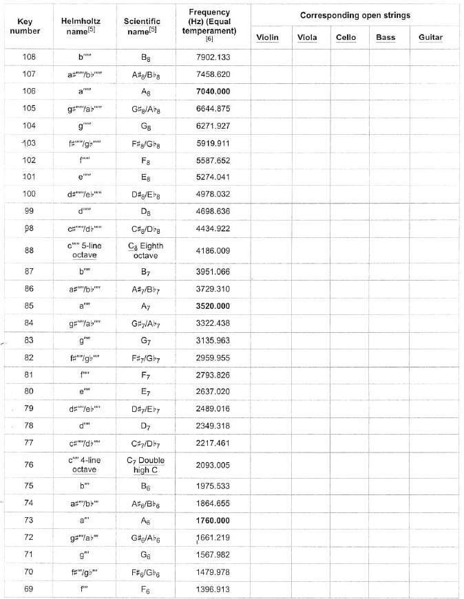

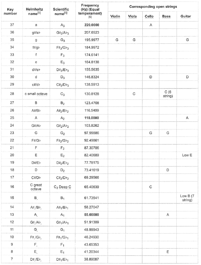
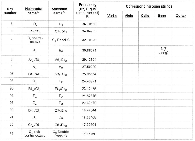
External Links
interactive piano frequency table (http://shakahara.com/pianopitch2.php) – A PHP script allowing the reference pitch of A4 to be altered from 440 Hz.
PySynth (https://web.archive.org/web/20190510200224/https://mdoege.github.io/PySynth/) – A simple Python-based software synthesizer that prints the key frequencies table and then creates a few demo songs based on that table.
“Keyboard and frequencies (http://www.sengpielaudio.com/calculator-notenames.htm)”, SengpielAudio.com.
Notefreqs (http://www.deimos.ca/notefreqs) – A complete table of note frequencies and ratios for midi, piano, guitar, bass, and violin. Includes fret measurements (in cm and inches) for building instruments.
Solution:
For a free-free beam the natural frequencies are found from:
![\[\cosh(kL)\cos(kL) = 1\]](https://engcourses-uofa.ca/wp-content/ql-cache/quicklatex.com-19585f9c99d5d935fed084e920cba372_l3.png "Rendered by QuickLaTeX.com")
and therefore  is a solution corresponding to a rigid body mode with no oscillation. The first mode is with
  and the frequency in Hz is:
![\[f_1 = \frac{(4.73)^2}{2\pi L^2} \sqrt{\frac{EI}{m}}\]](https://engcourses-uofa.ca/wp-content/ql-cache/quicklatex.com-3988e0592fc4ef7b19daea8c99409439_l3.png "Rendered by QuickLaTeX.com")
where  = modulus of elasticity, I section moment of area of the X section (bending), m = mass/unit length & L is the length of the beam for annulus
  sections
a) For the copper tubing
b)
![\[m = \frac{0.328}{12 \times 386} \frac{\text{lb} -\text{sec}^2}{\text{in}^2}\]](https://engcourses-uofa.ca/wp-content/ql-cache/quicklatex.com-484d720e5c4bdf7e9458fbfc933f5082_l3.png "Rendered by QuickLaTeX.com")
![\[E = 23 \times 10^6\]](https://engcourses-uofa.ca/wp-content/ql-cache/quicklatex.com-4c95b861cfbe337a999bf1644add23ba_l3.png "Rendered by QuickLaTeX.com")
c)
![\[I = \frac{\pi}{64}((0.875)^4 - (0.811)^4) = 5.297 \times 10^{-3} \text{m}^4\]](https://engcourses-uofa.ca/wp-content/ql-cache/quicklatex.com-38e0667adfaa633576b359ff786c97eb_l3.png "Rendered by QuickLaTeX.com")
For the 10 inch tube:
![\[\begin{split} f_1 &= \frac{22.373}{2\pi (10)^2} \sqrt{\frac{23 \times 10^6 \times 5.297 \times 10^{-3} \times 12 \times 386}{0.328}} \\&= 1477 \text{Hz} \end{split}\]](https://engcourses-uofa.ca/wp-content/ql-cache/quicklatex.com-fb242e3caed0abafa2a8abbf1d804bfe_l3.png "Rendered by QuickLaTeX.com")
as the other tubes are the dimension except for length
| Length (m) | Hang Pt / Length Ratio | Musical Pitch(Hz) | Musical Pitch (Desig) | Key |
| 8 7/8 | 0.225 | 1875 | A# | 74 |
| 9 7/16 | 0.225 | 1658 | G# | 72 |
| 10 | 0.225 | 1477 | F# | 70 |
| 10 7/8 | 0.224 | 1248 | D# | 67 |
| 11 1/2 | 0.223 | 1117 | C# | 65 |
The hang point corresponds to the nodal point of the fundamental frequency mode shape as shown.