
Review of single and multi-degree of freedom (mdof) systems: Applications of MDOF systems
The concept of modes and their corresponding natural frequencies is useful in understanding the behavior of lightly damped systems. Before adding the complication of damping to our models, we will consider several applications to industrial situations.
Example
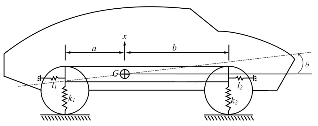
The model of the automobile shown is used to predict the low frequency modes of vibrations as these are responsible for the low frequency noise in the passenger compartment. Knowing these models can assist the designer in controlling them. In addition, it helps the designer in predicting the response of the frame to various inputs from road irregularities. As an initial estimate, the three modes of vibration of the vehicle may be considered as uncoupled. For the specific case below, the assumption of uncoupled modes is to be compared to the coupled model.
a) For the longitudinal model of the vehicle, specialize the equations of motion for the case of  (see previous section).
b) If any of the modes are uncoupled determine an expression of the natural frequency. For the coupled modes derive the equations of motion for free vibration starting from Newton’s laws.
c) Calculate the natural frequencies and mode shapes for the two coupled modes of vibration. The weight of the vehicle is  and the radius of gyration on the vehicle about
  is
is  .
.
Solution
a)
![\[ \begin{bmatrix} m & 0 & 0 \\ 0 & m & 0 \\ 0 & 0 & J_G \end{bmatrix}\begin{Bmatrix} \ddot{x} \\ \ddot{y} \\ \ddot{\theta} \end{Bmatrix} + \begin{bmatrix} \ell_1 + \ell_2 & 0 & 0 \\ 0 & k_1 + k_2 & k_2b - k_1a \\ 0 & k_2b-k_1a & k_1a^2 + k_2b^2 \end{bmatrix}\begin{Bmatrix} x \\ y \\ \theta \end{Bmatrix} = \begin{Bmatrix} 0 \\ 0 \\ 0 \end{Bmatrix} (+)\]](https://engcourses-uofa.ca/wp-content/ql-cache/quicklatex.com-89f3ea6139fd352075249f450fb6dd0e_l3.png "Rendered by QuickLaTeX.com")
b)
For horizontal motion:
![\[ m\ddot{x} + (\ell_1 + \ell_2)x = 0 \qquad \mathrm{ (uncoupled) }\]](https://engcourses-uofa.ca/wp-content/ql-cache/quicklatex.com-8755adcd3cd29bf86d7fd7833d9f3ed1_l3.png "Rendered by QuickLaTeX.com")
Therefore:
![\[ p_H = \sqrt{\frac{\ell_1 + \ell_2}{m}} \]](https://engcourses-uofa.ca/wp-content/ql-cache/quicklatex.com-80d014513506adba67f3e4dcafd7241d_l3.png "Rendered by QuickLaTeX.com")
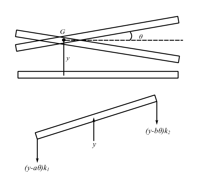
![\[ \begin{split} + \uparrow \sum F_y = & m\ddot{y} = -k_2(y+b\theta) - k_1(y-a\theta) \\ & m\ddot{y} + (k_1 + k_2)y + (k_2b-k_1a)\theta = 0 \qquad (I) \end{split}\]](https://engcourses-uofa.ca/wp-content/ql-cache/quicklatex.com-236115e096c075d86eece077cc215c3c_l3.png "Rendered by QuickLaTeX.com")
![\[ \begin{split}+\circlearrowleft \sum M_G =& J_G\ddot{\theta} = k_1a(y - a\theta) - k_2b(y+b\theta) \\ & J_G\ddot{\theta} + (k_2b-k_1a)y + (k_1a^2+k_2b^2)\theta \qquad (II) \end{split}\]](https://engcourses-uofa.ca/wp-content/ql-cache/quicklatex.com-a218dbdcd533f23d3b3f0a6ced0b9b11_l3.png "Rendered by QuickLaTeX.com")
 &
&  are the same as
  .
.
c)
![\[ \omega = 3550 \ \text{lbs} \]](https://engcourses-uofa.ca/wp-content/ql-cache/quicklatex.com-70d2f5577967781a08e45544c8ac36ea_l3.png "Rendered by QuickLaTeX.com")
![\[a = 4.5\ \text{ft}\]](https://engcourses-uofa.ca/wp-content/ql-cache/quicklatex.com-f27facc46cb0cdace391ba2c8d48fd23_l3.png "Rendered by QuickLaTeX.com")
![\[b = 5.5 \ \text{ft}\]](https://engcourses-uofa.ca/wp-content/ql-cache/quicklatex.com-5dfcefd4cdf0b9d81d85aba0e8cfcc8f_l3.png "Rendered by QuickLaTeX.com")
![\[\bar{r} = 4 \ \text{ft}\]](https://engcourses-uofa.ca/wp-content/ql-cache/quicklatex.com-872cbf836c55eb1a82f19732e20a188f_l3.png "Rendered by QuickLaTeX.com")
![\[k_1 = 2200 \ \text{lb/ft}\]](https://engcourses-uofa.ca/wp-content/ql-cache/quicklatex.com-066794defeb514110727b0c69703b33b_l3.png "Rendered by QuickLaTeX.com")
![\[k_2 = 2700 \ \text{lb/ft}\]](https://engcourses-uofa.ca/wp-content/ql-cache/quicklatex.com-129a53a01a4ad14403dbcb6f4f7c3873_l3.png "Rendered by QuickLaTeX.com")
Therefore:
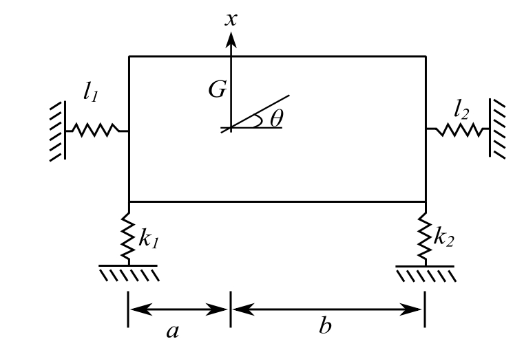
![\[\begin{bmatrix} m & 0 \\ 0 & J_G \end{bmatrix} \begin{Bmatrix} \ddot{x} \\ \ddot{\theta} \end{Bmatrix} + \begin{bmatrix} k_1 + k_2 & k_2b - k_1a \\ k_2b - k_1a & k_1a^2 +k_2b^2 \end{bmatrix} \begin{Bmatrix} x \\ \theta \end{Bmatrix} = \begin{Bmatrix} 0 \\ 0 \end{Bmatrix} \]](https://engcourses-uofa.ca/wp-content/ql-cache/quicklatex.com-133249c6ece27965f41f85355df01ec7_l3.png "Rendered by QuickLaTeX.com")
Assume  :
:
![\[\begin{bmatrix} (k_1 + k_2) - mp^2 & k_2b-k_1a \\ k_2b - k_1a & k_1a^2 + k_2b^2 - J_Gp^2 \end{bmatrix} \begin{Bmatrix} X \\ \Theta \end{Bmatrix} = 0 \]](https://engcourses-uofa.ca/wp-content/ql-cache/quicklatex.com-34f482dfa018557d303b2862ed321a82_l3.png "Rendered by QuickLaTeX.com")
![\[ [k_1 + k_2 -mp^2][k_1a^2+k_2b^2-J_Gp^2] - (k_2b - k_1a)^2 = 0 \]](https://engcourses-uofa.ca/wp-content/ql-cache/quicklatex.com-c0bac554ae0c763ec3de6e4aae02f91d_l3.png "Rendered by QuickLaTeX.com")
![\[(k_1+k_2)(k_1a^2+k_2b^2)-p^2\big[J_G(k_1+k_2)+(k_1a^2+k_2b^2)m\big]+mJ_Gp^4-(k_2b-k_1a)^2 =0 \]](https://engcourses-uofa.ca/wp-content/ql-cache/quicklatex.com-c4e52f434c2e9e0d361de16403287ebd_l3.png "Rendered by QuickLaTeX.com")
![\[mJ_Gp^4-mp^2\big[\vec{r}^2(k_1+k_2)+(k_1a^2+k_2b^2)\big]+[(k_1+k_2)(k_1a^2+k_2b^2)]-(k_2b-k_1a)^2 = 0 \]](https://engcourses-uofa.ca/wp-content/ql-cache/quicklatex.com-87ea8667dafec0b298772baadc747a72_l3.png "Rendered by QuickLaTeX.com")
![\[p^4-p^2\bigg[\frac{k_1+k_2}{m}+\frac{(k_1a^2+k_2b^2)}{m\vec{r}^2}\bigg]+\bigg(\frac{k_1+k_2}{m}\bigg)\bigg(\frac{k_1a^2+k_2b^2}{m\vec{r}^2}\bigg)-\frac{(k_2b-k_1a)^2}{mm\vec{r}^2} = 0 \]](https://engcourses-uofa.ca/wp-content/ql-cache/quicklatex.com-99db155d1f9f49a2f80bbfd962bea29e_l3.png "Rendered by QuickLaTeX.com")
![\[p^4-p^2[44.45+74.99]+(44.45)(74.99)-126.0 =0 \]](https://engcourses-uofa.ca/wp-content/ql-cache/quicklatex.com-e2259ab2cb9cbb2f2a48ea6f12aa4bbc_l3.png "Rendered by QuickLaTeX.com")
![\[p^4-119.44p^2+3207 = 0 \]](https://engcourses-uofa.ca/wp-content/ql-cache/quicklatex.com-0aae60a0f1680bf41b03d3dcc6906e94_l3.png "Rendered by QuickLaTeX.com")
![\[p^2 =\frac{119.44}{2}\pm \sqrt{\left(\frac{119.44}{2}\right)^2-3207} = 59.7 \pm 18.96 \]](https://engcourses-uofa.ca/wp-content/ql-cache/quicklatex.com-520ca1756fe5433f1bbbe64ed5a5f7f9_l3.png "Rendered by QuickLaTeX.com")
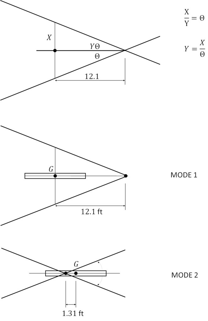
![\[\begin{split} p_1^2 &=40.74 \\ p_2^2 &=78.65 \\ p_{1,2} &= 6.38 \ \text{rads/s}, 8.87 \ \text{rads/s} \\ &= \underline{\underline{1.01 \ \text{Hz}}}, \underline{\underline{1.41 \ \text{Hz}}} \end{split}\]](https://engcourses-uofa.ca/wp-content/ql-cache/quicklatex.com-cf95d1f33f0b64224130b7c6bc34721d_l3.png "Rendered by QuickLaTeX.com")
![\[(k_1+k_2-mp^2)X + (k_2b-k_1a)\Theta = 0 \]](https://engcourses-uofa.ca/wp-content/ql-cache/quicklatex.com-62528f419a00460aa8526d3ba1bde6de_l3.png "Rendered by QuickLaTeX.com")
![\[\begin{split} \frac{X}{\Theta} &= \frac{(k_1a-k_2b)}{k_1+k_2-mp^2} \\ & \\ \Big(\frac{X}{\Theta}\Big)_1 &= \frac{(k_1a-k_2b)/m}{\frac{(k_1+k_2)}{m}-p^2} \\ &= \frac{[(2200)(45)-2700(5.5)]\frac{32.2}{3550}}{(44.45)-40.74} \\ &= \underline{\underline{-12.1 \ \text{ft/rad}}} \\ & \\ \Big(\frac{X}{\Theta}\Big)_2 &= \frac{-44.90}{44.45-78.65} \\ &= \underline{\underline{1.31}} \text{ft/rad}\end{split}\]](https://engcourses-uofa.ca/wp-content/ql-cache/quicklatex.com-bb4130f76f47c5756552b38bc48f1e1d_l3.png "Rendered by QuickLaTeX.com")
If we “uncoupled” the modes
Assume vertical node is
![\[\begin{split} p_1 &= \sqrt{\frac{k_1+k_2}{m}} \\ &= \sqrt{\frac{4900*32.3}{3550}} \\ &= 6.67 \ \text{rads/s} \\ &= \underline{\underline{1.06 \ \text{Hz}}} \end{split}\]](https://engcourses-uofa.ca/wp-content/ql-cache/quicklatex.com-aae8a518ff8f459e17462de1a0406d1e_l3.png "Rendered by QuickLaTeX.com")
Rotational Mode
![\[\begin{split} p_2 &=\sqrt{\frac{k_1a^2+k_2b^2}{m\vec{r}^2}} \\ &= \sqrt{\frac{[(2200)(4.5)^2+(2700)(5.5)^2]32.2}{3550(4)^2}} \\ &= 8.46 \ \text{rads/s} \\ &= \underline{\underline{1.35 \ \text{Hz}}} \end{split}\]](https://engcourses-uofa.ca/wp-content/ql-cache/quicklatex.com-60c99da2cc7ed2fc374705243466c3a1_l3.png "Rendered by QuickLaTeX.com")
If the horizontal stiffness,  , were the same as the vertical then the third frequency,
  , would be the same as the vertical.
The assumption of uncoupling gives essentially the same answer.
Example
The illustration shows the detail of the proposed isolation system for the reciprocating compressor and motor considered previously and modelled as a single dof system. The actual system does not have the center of gravity symmetrically located on the supporting structure and isolation springs. In situations like these the industrial installation guides recommend that the isolation springs be selected so that the vertical static deflection of all springs is the same. The reason stated is that this will tend to reduce the frequency of the “rocking motions”. This exercise is to investigate this idea as well as the differences found for the isolation of the system compared with the single degree approximation used earlier. More details of the installation are given below. The stiffnesses shown are representative of both springs at the ends of the supports with the lateral stiffnesses assumed to be equal to the vertical values.
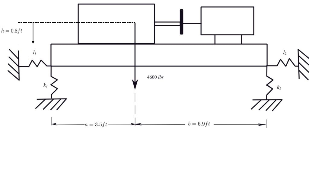
a) If the vertical static deflection of the spring is the same what is the ratio of  and
and  ?
?
![\[ S_1 = \frac{F_1}{k_1}, \ S_2=\frac{F_2}{k_2} \]](https://engcourses-uofa.ca/wp-content/ql-cache/quicklatex.com-e6917a603cc7bf038f83296e97fab833_l3.png "Rendered by QuickLaTeX.com")
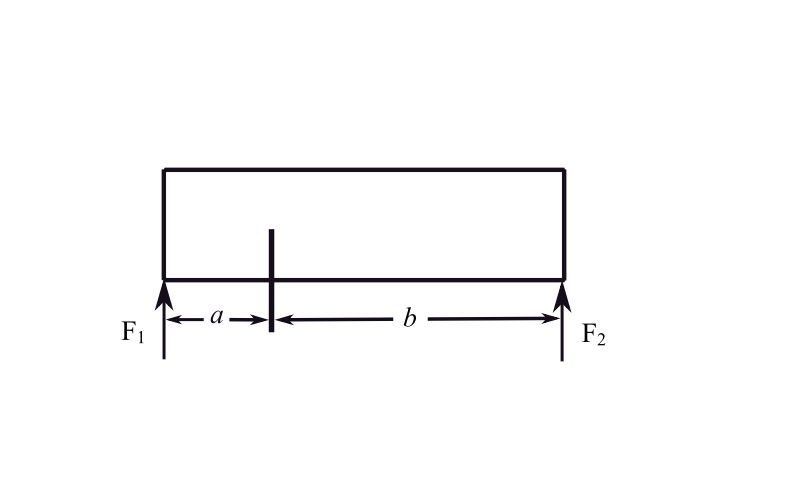
For static equilibrium
![\[\begin{split} F_1a &=F_2b \\ \frac{F_1}{k_1} &= \frac{F_1(\frac{a}{b})}{k_2} \end{split} \]](https://engcourses-uofa.ca/wp-content/ql-cache/quicklatex.com-6a43609dc24704c42f0bf596031757dc_l3.png "Rendered by QuickLaTeX.com")
therefore:
![\[\begin{split} \frac{k_2}{k_1} &=\frac{a}{b} \\ k_2b &= k_1a \end{split} \]](https://engcourses-uofa.ca/wp-content/ql-cache/quicklatex.com-f843b0cf598cf7b6822ca311d00c2224_l3.png "Rendered by QuickLaTeX.com")
(b) Under this assumption what happens to the equations of motion?
![\[\begin{bmatrix} m & 0 & 0 \\0 & m & 0 \\ 0 & 0 & m\vec{r}^2 \end{bmatrix}\begin{Bmatrix}\Ddot{x} \\ \Ddot{y} \\ \Ddot{\theta}\end{Bmatrix} + \begin{bmatrix} \ell_1 + \ell_2 & 0 & (\ell_1+\ell_2)h \\0 & k_1+k_2 & 0 \\(\ell_1+\ell_2)h & 0 & h^2(\ell_1+\ell_2)+k_1a^2+k_2b^2\end{bmatrix}\begin{Bmatrix}x \\ y \\ \theta\end{Bmatrix} = \begin{Bmatrix}0\end{Bmatrix}\]](https://engcourses-uofa.ca/wp-content/ql-cache/quicklatex.com-9d30ddb78329ba918b26732662ebf1bf_l3.png "Rendered by QuickLaTeX.com")
as the vertical mode is uncoupled from the other two
![\[ p_v = \sqrt{\frac{k_1+k_2}{m}} \]](https://engcourses-uofa.ca/wp-content/ql-cache/quicklatex.com-8bc176651a14fe8809e0399e5a795456_l3.png "Rendered by QuickLaTeX.com")
becomes
![\[\begin{bmatrix}m & 0 \\ 0 & mr^2\end{bmatrix}\begin{Bmatrix}\Ddot{x} \\ \Ddot{\theta}\end{Bmatrix} + \begin{bmatrix}\ell_1+\ell_2 & (\ell_1+\ell_2)h \\(\ell_1+\ell_2)h & h^2(\ell_1+\ell_2)+k_1a^2+k_2b^2\end{bmatrix}\begin{Bmatrix}x \\ \theta\end{Bmatrix}=\begin{Bmatrix}0\end{Bmatrix}\]](https://engcourses-uofa.ca/wp-content/ql-cache/quicklatex.com-61b94e5b76fbcc61c1f6c67b9912ba38_l3.png "Rendered by QuickLaTeX.com")
(c) Noting that the original had an operating speed of 1750 RPM and the original transmissibility was 1/15, calculate  for this installation assuming
![\[ \frac{1}{(\frac{\omega}{p_v})^2-1}=\frac{1}{15} \]](https://engcourses-uofa.ca/wp-content/ql-cache/quicklatex.com-48dde5f8c485e9f8629f719739da1c63_l3.png "Rendered by QuickLaTeX.com")
therefore:
![\[ \begin{split} \frac{\omega}{p_v} &=4 \\ p_v &=\frac{1750}{4} \\ &=437.5 \ \text{RPM} \\ &= \frac{437.5*2\pi}{60} \\ &=45.8 \ \text{rads/s} \\ &=7.3 \ \text{Hz} \end{split} \]](https://engcourses-uofa.ca/wp-content/ql-cache/quicklatex.com-eafc539344342a66674b56d4d835e3d9_l3.png "Rendered by QuickLaTeX.com")
therefore:
![\[\begin{split} \sqrt{\frac{(k_1+k_2)32.2}{4600}} &=45.8 \\ k_1 + k_2 &= (45.8)^2\frac{4600}{32.2} \\ &=300,000 \text{ lb/ft} \end{split}\]](https://engcourses-uofa.ca/wp-content/ql-cache/quicklatex.com-7c9a35a25a517f1b175a265dc0c1de3d_l3.png "Rendered by QuickLaTeX.com")
therefore:
![\[\begin{split}k_1+k_1\frac{a}{b} &=k_1\Big(1+\frac{3.5}{6.9}\Big) \\ &=300,000 \text{ lbs/ft} \end{split}\]](https://engcourses-uofa.ca/wp-content/ql-cache/quicklatex.com-f06183740d95c3ca57185cf16026938f_l3.png "Rendered by QuickLaTeX.com")
![\[k_1=\frac{300,000}{1.65217}=181,600 \ \text{lbs/ft}\]](https://engcourses-uofa.ca/wp-content/ql-cache/quicklatex.com-2d44aa70917ab24f292578f6ae05c5aa_l3.png "Rendered by QuickLaTeX.com")
![\[k_2 = 0.65217\cdot181,600 = \ \underline{\underline{\text{118,400 lbs/ft}}}\]](https://engcourses-uofa.ca/wp-content/ql-cache/quicklatex.com-d784e55bbb2f5b7daa956ec068587f45_l3.png "Rendered by QuickLaTeX.com")
(d) Assuming SSHM
![\[\begin{Bmatrix}x \\ \theta\end{Bmatrix}= \begin{bmatrix}X \\ \Theta\end{bmatrix}\sin(pt+\phi)\]](https://engcourses-uofa.ca/wp-content/ql-cache/quicklatex.com-6d8c0b88785fba6daaea5b335febea65_l3.png "Rendered by QuickLaTeX.com")
![\[ \begin{bmatrix}\ell_1+\ell_2-mp^2 & (\ell_1+\ell_2)h \\(\ell_1+\ell_2)h & h^2(\ell_1+\ell_2)+k_1a^2+k_2b^2-mr^2p^2\end{bmatrix}\begin{Bmatrix}X \\ \Theta\end{Bmatrix}= \begin{Bmatrix}0\end{Bmatrix}\]](https://engcourses-uofa.ca/wp-content/ql-cache/quicklatex.com-1b461b2dbba3a1d388447ddf489a9e43_l3.png "Rendered by QuickLaTeX.com")
![\[(r = \text{radius of gyration})\]](https://engcourses-uofa.ca/wp-content/ql-cache/quicklatex.com-05b0d6b109e9b24888feb337ad8a4179_l3.png "Rendered by QuickLaTeX.com")
therefore:
![\[ \Big[\ell_1+\ell_2-mp^2\Big]\Big[h^2(\ell_1+\ell_2)+k_1a^2+k_2b^2-mr^2p^2\Big]-(\ell_1+\ell_2)^2h^2 = 0\]](https://engcourses-uofa.ca/wp-content/ql-cache/quicklatex.com-f60028b5336bbe6e014239e0ca8e1133_l3.png "Rendered by QuickLaTeX.com")
Divide by
 to get
 ![\[ \biggr[\frac{\ell_1+\ell_2}{m}-p^2\biggr]\biggr[\frac{(\ell_1+\ell_2)}{m}\frac{h^2}{r^2}+\frac{k_1}{m}\frac{a^2}{r^2}+\frac{k_2}{m}\frac{b^2}{r^2}-p^2\biggr]-\frac{(\ell_1+\ell_2)^2}{m^2}\frac{h^2}{r^2} = 0\]](https://engcourses-uofa.ca/wp-content/ql-cache/quicklatex.com-4442395d2fe2904193120bcbc583f992_l3.png "Rendered by QuickLaTeX.com")
therefore:
![\[\begin{split}p^4 &-p^2\biggr[\frac{\ell_1+\ell_2}{m}+\frac{\ell_1+\ell_2}{m}\frac{h^2}{r^2}+\frac{k_1}{m}\frac{a^2}{r^2}+\frac{k_2}{m}\frac{b^2}{r^2}\biggr] \\ &+ \frac{(\ell_1+\ell_2)^2}{m^2}\frac{h^2}{r^2} + \frac{(\ell_1+\ell_2)}{m}(\frac{k_1}{m}\frac{a^2}{r^2}+\frac{k_2}{m}\frac{b^2}{r^2}) - \frac{(\ell_1+\ell_2)^2}{m^2}\frac{h^2}{r^2} = 0 \end{split}\]](https://engcourses-uofa.ca/wp-content/ql-cache/quicklatex.com-208897f2f60de7b28a26e512a06ef16b_l3.png "Rendered by QuickLaTeX.com")
![\[p^4-p^2\biggr[\Big(\frac{\ell_1+\ell_2}{m}\Big)\Big(1+\frac{h^2}{r^2}\Big)+\frac{(k_1a^2+k_2b^2)}{mr^2}\biggr] + \frac{(\ell_1+\ell_2)(k_1a^2+k_2b^2)}{m^2r^2} = 0\]](https://engcourses-uofa.ca/wp-content/ql-cache/quicklatex.com-275146477188b9034b650d5629cd7742_l3.png "Rendered by QuickLaTeX.com")
![\[ \begin{split}p^4 &-p^2\biggr[\frac{(300,000)}{4600}\Big(1+\Big(\frac{0.8}{2.1}\Big)\strut^2\Big)32.2+\frac{181,600}{4600}\Big(\frac{3.5}{2.1}\Big)\strut^2\Big(32.2\Big)+\frac{118,400}{4600}\Big(\frac{6.9}{2.1}\Big)\strut^2 32.2\biggr] \\ &+ \frac{300,000}{(4600)^2}\biggr[181,600\Big(\frac{3.5}{2.1}\Big)\strut^2+118,400\Big(\frac{6.9}{2.1}\Big)\strut^2\biggr](32.2)^2 = 0\end{split} \]](https://engcourses-uofa.ca/wp-content/ql-cache/quicklatex.com-3d40fb8bc46385e727ea5f4f6f924b6e_l3.png "Rendered by QuickLaTeX.com")
![\[ \begin{split} p^2 &= 7470 \pm 5429 \\ & \\ p_1 &= 45.2 \ \text{rads/s (7.2 Hz)} \\ p_2 &= 113.6 \ \text{rad/s (18.1 Hz)} \end{split}\]](https://engcourses-uofa.ca/wp-content/ql-cache/quicklatex.com-be4682a49c5f9168493d6462c6824f0a_l3.png "Rendered by QuickLaTeX.com")
(e)
![\[ \begin{split} p_v &= 45.8 \ \text{rads/s (7.3 Hz)} \\ p_H &= 45.8 \text{rads/s (7.3 Hz)} \end{split} \]](https://engcourses-uofa.ca/wp-content/ql-cache/quicklatex.com-f208f9da7bc4a4008eafc19939b59ba2_l3.png "Rendered by QuickLaTeX.com")
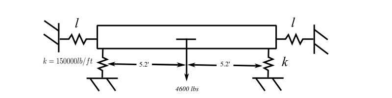
The rotational mode can be calculated starting from a FBD
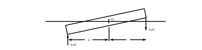
![\[\begin{split} \Sigma M_G &= m\vec{r}^2\Ddot{\theta} \\ &= -ka^2\theta - ka^2\theta \end{split} \]](https://engcourses-uofa.ca/wp-content/ql-cache/quicklatex.com-e2ac01adeb4349fc3573cb296893bfe3_l3.png "Rendered by QuickLaTeX.com")
therefore:
![\[ \begin{split} P^2_{\theta} &= \frac{2ka^2}{mr^2} \\ &= \frac{300,000(5.2)^2(32.2)}{4600(2.1)^2} \end{split}\]](https://engcourses-uofa.ca/wp-content/ql-cache/quicklatex.com-0f3d495dd21050dbece95316cf32644a_l3.png "Rendered by QuickLaTeX.com")
![\[ \begin{split} P_{\theta} &= 113.5 \ \text{rads/s} \\ &= (18.1 \ \text{Hz}) \end{split} \]](https://engcourses-uofa.ca/wp-content/ql-cache/quicklatex.com-0d41efd4dd512c06f2d9992a37c10e52_l3.png "Rendered by QuickLaTeX.com")
(f) Do the calculation using a program
(g) From d)
![\[ \begin{split} p_v &=7.3 \ \text{Hz} \\ (p_H)_1 &= 7.2 \ \text{Hz} \\ (p_{\theta})_2 &= 18.1 \ \text{Hz} \end{split} \]](https://engcourses-uofa.ca/wp-content/ql-cache/quicklatex.com-fc6ccb181bd14d64edcd0dcb6958fc76_l3.png "Rendered by QuickLaTeX.com")
from e)
![\[ \begin{split} p_v &= 7.3 Hz \\ p_H &= 7.3 Hz \\ p_{\theta} &= 18.1 Hz \end{split} \]](https://engcourses-uofa.ca/wp-content/ql-cache/quicklatex.com-1c765d5e195ff77b30a5b669eb1afbe5_l3.png "Rendered by QuickLaTeX.com")
from (f)
![\[ \begin{split} (p)_{v_1} &= ? \\ (p_H)_2 &= ? \\ (p_{\theta})_3 &= ? \end{split} \]](https://engcourses-uofa.ca/wp-content/ql-cache/quicklatex.com-36f8c7270a1d44cbc06c9b9b4ac22b50_l3.png "Rendered by QuickLaTeX.com")
The results show that because  is small compared to
  and
and  that there is little difference. The “rotational” (
 ) is very much higher than the other two and closer to the excitation frequency of 29.2 Hz (1750 RPM).
To lower it, the spacing of the supports would have to be reduced. For example if it were brought to 1/2 of original (5.1′ instead of a total of 10.4′) then the rotational natural frequency would be
![\[ p_{\theta} = \sqrt{\frac{300,000(2.6)^2(32.2)}{4600(2.1)^2}} = 56.7 \ \text{rads/s} \]](https://engcourses-uofa.ca/wp-content/ql-cache/quicklatex.com-21541cfcdebd2a56173b377afdaac5a7_l3.png "Rendered by QuickLaTeX.com")
It is obvious from this calculation that the rule of thumb should be that the spacing should be no more than twice the radius of gyration of the total mass!
Example
A commercial front loading washing machine is being used by a spa located adjacent to a medical clinic in a strip mall. During the spin cycle of the washing machine the fluctuating force due to the imbalance of the load causes the floor to vibrate and induces unacceptable levels of noise in the clinic. To reduce this disturbance, an engineering consultant recommends using spring isolation between the washing machine and the floor to reduce the dynamic force transmitted to 20% of the exciting force. The specifications of the washing machine are summarized below. Assume only vertical vibration and neglect damping.
| Net weight | 1049 lbs |
| Maximum load | 255lbs |
| Maximum Dynamic Force | 212 lbs |
| Spin Speed (Frequency of Dynamic Force) | 950 RPM (15.8 Hz) |
| Cylinder Diameter | 27.6 inch |
a) Calculate the appropriate spring constant for each of four springs used to mount the washing machine to meet the specification for the transmissibility and select them from the enclosed table.
b) This washing machine can also be run at a spin speed of 750 RPM. Calculate the Dynamic Force at this RPM and then calculate the force transmitted to the supporting structure compared with the force transmitted at 950 RPM.
c) Using the size of the rotating wash cylinder estimate the unbalanced weight in the maximum load.
| Mount No. | Mount Constant (  ) ) | Load at 2-in. Deflection (  ) ) |
| SLF-401 | 50 | 100 |
| SLF-402 | 70 | 140 |
| SLF-403 | 90 | 180 |
| SLF-404 | 115 | 230 |
| SLF-405 | 150 | 300 |
| SLF-406 | 200 | 400 |
| SLF-407 | 305 | 610 |
| SLF-408 | 365 | 730 |
| SLF-409 | 500 | 1,000 |
| SLF-410 | 650 | 1,300 |
| SLF-411 | 740 | 1,880 |
| SLF-412 | 1,150 | 2,300 |
| SLF-413 | 1,500 | 3,000 |
| SLF-414 | 2,000 | 4,000 |
| SLF-415 | 2,680 | 5,360 |
| SLF-416 | 3,500 | 7,000 |
| SLF-417 | 4,750 | 9,500 |
| SLF-418 | 6,250 | 12,500 |
| SLF-419 | 8,200 | 16,400 |
| SLF-420 | 11,250 | 22,500 |
| SLF-421 | 15,000 | 30,000 |
| SLF-422 | 20,000 | 40,000 |
a)
![\[M = \frac{1049+255}{386}\]](https://engcourses-uofa.ca/wp-content/ql-cache/quicklatex.com-b1833e132547df5aea212b37dee22bdb_l3.png "Rendered by QuickLaTeX.com")
![\[\begin{split} T &= 0.2 \\&= \frac{1}{(\frac{\omega}{p})^2-1} \end{split}\]](https://engcourses-uofa.ca/wp-content/ql-cache/quicklatex.com-da32275cc0d05a7efcc311c84cda7fc7_l3.png "Rendered by QuickLaTeX.com")
Therefore,
![\[\frac{\omega^{2}}{p^{2}} = 5\]](https://engcourses-uofa.ca/wp-content/ql-cache/quicklatex.com-20d67a466e62db54656e67eabdea8bc3_l3.png "Rendered by QuickLaTeX.com")
![\[\begin{split} \frac{\omega}{p} &= \sqrt{6} \\&= 2.44 \end{split}\]](https://engcourses-uofa.ca/wp-content/ql-cache/quicklatex.com-e9537b3bc663690a9bd2d40af75ef91e_l3.png "Rendered by QuickLaTeX.com")
![\[\begin{split} p &= \frac{\omega}{\sqrt{6}} \\&= \frac{950\cdot(2 \pi)}{60 \sqrt{6}} \\&= 40.61 \ \text{rad/s} \end{split}\]](https://engcourses-uofa.ca/wp-content/ql-cache/quicklatex.com-5759ee74bb73d1f2809a9c72d09b3c33_l3.png "Rendered by QuickLaTeX.com")
![\[\begin{split} k &= p^{2}M = (40.61)^{2} \\&= (40.61)^{2}\Big(\frac{1304}{386}\Big) \\&= 5571.3 \ \text{lb/in} \end{split}\]](https://engcourses-uofa.ca/wp-content/ql-cache/quicklatex.com-fc316d5c30743d13d53f3d777cf2d612_l3.png "Rendered by QuickLaTeX.com")
Therefore, each spring has
![\[\begin{split} k &= \frac{5571.3}{4} \\&= 1393 \ \text{lbs/in} \end{split}\]](https://engcourses-uofa.ca/wp-content/ql-cache/quicklatex.com-2b2e2e78f54f8a38f4b43d01de56f08a_l3.png "Rendered by QuickLaTeX.com")
Therefore, SLF 412 as 413 would not meet the transmissibility spec.
b)
![\[\omega_{950} = \sqrt{6}p\]](https://engcourses-uofa.ca/wp-content/ql-cache/quicklatex.com-34f1b52575f8f43db00e924e1f688f88_l3.png "Rendered by QuickLaTeX.com")
![\[\omega_{750} = \sqrt{6}p \Big(\frac{750}{950}\Big)\]](https://engcourses-uofa.ca/wp-content/ql-cache/quicklatex.com-a73618956d04f98d970e8a89253da2b9_l3.png "Rendered by QuickLaTeX.com")
![\[\frac{\omega}{p}_{750} = \sqrt{6}\Big(\frac{750}{950}\Big)\]](https://engcourses-uofa.ca/wp-content/ql-cache/quicklatex.com-09b3fc92e837b937ea3187f653d986d9_l3.png "Rendered by QuickLaTeX.com")
![\[\begin{split} T_{750} &= \frac{1}{6\big(\frac{75}{95}\big)^{2}-1} \\&= 0.365 \end{split}\]](https://engcourses-uofa.ca/wp-content/ql-cache/quicklatex.com-93cff2962633aed80ed05048034de538_l3.png "Rendered by QuickLaTeX.com")
![\[T_{950} = 0.2\]](https://engcourses-uofa.ca/wp-content/ql-cache/quicklatex.com-1761b282b2273f2f11ae464e23d853ac_l3.png "Rendered by QuickLaTeX.com")
![\[F_{o-950} = 212\ \text{lbs}\]](https://engcourses-uofa.ca/wp-content/ql-cache/quicklatex.com-e60443dc26ae1a7b4e33bb695e7d31f5_l3.png "Rendered by QuickLaTeX.com")
![\[\begin{split} F_{o-750} &= 212\Big(\frac{75}{96}\Big)^{2} \\&= 132\ \text{lbs} \end{split}\]](https://engcourses-uofa.ca/wp-content/ql-cache/quicklatex.com-3d5be0441e0aa19bd58fa5920ffbe8a2_l3.png "Rendered by QuickLaTeX.com")
![\[\begin{split} F_{T-950} &= 212\cdot0.2 \\&= 42 \ \text{lbs} \end{split}\]](https://engcourses-uofa.ca/wp-content/ql-cache/quicklatex.com-f0347fead62b3ef64d17fd934aba7a4c_l3.png "Rendered by QuickLaTeX.com")
![\[\begin{split} F_{T-750} &= 132\cdot0.365 \\&= 48 \ \text{lbs} \end{split}\]](https://engcourses-uofa.ca/wp-content/ql-cache/quicklatex.com-8c6233fc6ce1d06291d453eb5cd8f459_l3.png "Rendered by QuickLaTeX.com")
Therefore slightly higher than at 950 RPM
c)
![\[\begin{split} \text{Dynamic Force} &= \tilde{m}e\omega^{2} \\&= \frac{W_{im}}{g}e\omega^{2} \\&= \frac{W_{im}}{386}(13.8)(15.2\cdot2\pi)^{2} \\&= 212 \ \text{lbs} \end{split}\]](https://engcourses-uofa.ca/wp-content/ql-cache/quicklatex.com-3938b83a8e8ba7f06509d68e5b6702d2_l3.png "Rendered by QuickLaTeX.com")
![\[\begin{split} W_{im} &= \frac{(212)(386)}{(13.8)(15.2\cdot2\pi)^{2}} \\&= 0.60 \ \text{lbs} \end{split}\]](https://engcourses-uofa.ca/wp-content/ql-cache/quicklatex.com-a7c2a89e40a07986a11456f12602a8a5_l3.png "Rendered by QuickLaTeX.com")
Perhaps a wet hand towel out of balance
The commercial washer above was considered under the assumption that the vibration was only a vertical mode. However the excitation due to rotating imbalance would cause excitation both horizontally and vertically that would excite coupled modes as well. As a result it is necessary to consider all the planar modes of vibration to investigate if they are near the excitation frequency. The diagram of the dryer is shown below. The lateral stiffness of the supporting springs is estimated to be 0.8 of the vertical stiffness. The excitation frequency is 950 rpm.
![\[W = 1049+255 \ \text{lbs}\]](https://engcourses-uofa.ca/wp-content/ql-cache/quicklatex.com-16c3c3d27103021060249ec7132a3a3f_l3.png "Rendered by QuickLaTeX.com")
![\[\bar{r} = 15 \text{ in (radius of gyration)}\]](https://engcourses-uofa.ca/wp-content/ql-cache/quicklatex.com-8d2bcea2fd3699d098f8a11a830c0519_l3.png "Rendered by QuickLaTeX.com")
![\[k_1 = k_2 = k = 1150 \ \text{lbs/in}\]](https://engcourses-uofa.ca/wp-content/ql-cache/quicklatex.com-9a9b41e8daccccfbeee1fddbf49fa48d_l3.png "Rendered by QuickLaTeX.com")
![\[\ell_1 = \ell_2 = 0.8k \text{ (4 springs)}\]](https://engcourses-uofa.ca/wp-content/ql-cache/quicklatex.com-f346c040c3139ad67b6c7461cd430dd3_l3.png "Rendered by QuickLaTeX.com")
![\[h = 28 \ \text{in}\]](https://engcourses-uofa.ca/wp-content/ql-cache/quicklatex.com-2f32d93675b7cebb433bd9c785800eb6_l3.png "Rendered by QuickLaTeX.com")
![\[a = 19 \ \text{in}\]](https://engcourses-uofa.ca/wp-content/ql-cache/quicklatex.com-c1089163faf6ecbd660e8f0132728657_l3.png "Rendered by QuickLaTeX.com")
a) Specialize the equations of motion for the case shown in the above diagram
b) Determine if any of the modes are uncoupled. For the coupled modes derive the equations of motion for free vibration starting from Newton’s laws.
c) Calculate the natural frequencies and mode shapes for the dryer.
d) If the supports for the dryer were redesigned to make loading easier with h = 0 (as illustrated) what are the natural frequencies compared to the original design. How do they compare with the excitation frequency?
a)

b) Therefore  ,
,
The vertical mode is uncoupled
![\[\begin{split} \underrightarrow{+} \sum F_x &= m\ddot{x} \\&= -4\ell(x+h\theta) \end{split}\]](https://engcourses-uofa.ca/wp-content/ql-cache/quicklatex.com-ef039d5df36aa3e74b84c05848e54bdd_l3.png "Rendered by QuickLaTeX.com")
![\[\begin{split} + \circlearrowleft \sum M_G &= J_G \ddot{\theta} \\&= -4\ell(x+h\theta)h-2k(a\theta)a - 2k(a\theta)a \end{split}\]](https://engcourses-uofa.ca/wp-content/ql-cache/quicklatex.com-a0bda5b87234e3b011b7ac2d7a015da3_l3.png "Rendered by QuickLaTeX.com")
Therefore
![\[m\ddot{x} + 4kx + 4\ell h\theta = 0\]](https://engcourses-uofa.ca/wp-content/ql-cache/quicklatex.com-70e87e08a55921b046c21ba984c5b6d2_l3.png "Rendered by QuickLaTeX.com")
![\[J\ddot{\theta} + 4\ell hx+ (4\ell h^{2}+4ka^{2})\theta = 0\]](https://engcourses-uofa.ca/wp-content/ql-cache/quicklatex.com-d4847de9166f8716228b60c8c2de2972_l3.png "Rendered by QuickLaTeX.com")
Which matches the reduction of the general case where  has been replaced by
  and
and  by
by 
c) Calculate the natural frequencies and mode shapes for the dryer
The vertical mode is as previously
![\[\begin{split} p_v &= \sqrt{\frac{2k}{m}}_\text{eff} \\&= \sqrt{\frac{4\cdot1150\cdot386}{(1049+255)}} \\&= 36.90 \ \text{rad/s} \\&= 5.98 \ \text{Hz} \end{split}\]](https://engcourses-uofa.ca/wp-content/ql-cache/quicklatex.com-d62ed83fa96d9abe6f78c02c55c9d436_l3.png "Rendered by QuickLaTeX.com")
which is well below the excitation frequency of 950RPM (15.8Hz)

Assume that


![\[(4\ell-mp^{2})(4\ell h^{2} + 4ka^{2} - m\bar{r}^{2}p^{2}) - 16\ell^{2}h^{2} = 0\]](https://engcourses-uofa.ca/wp-content/ql-cache/quicklatex.com-5f1d5c25adf90e9cd7cab227d48f3756_l3.png "Rendered by QuickLaTeX.com")
![\[16\ell^{2}h^{2} + 16k\ell a^{2} - 4\ell \bar{r}^{2}p^{2}m- 4\ell h^{2}mp^{2} - 4ka^{2}mp^{2} + m\bar{r}^{2}p^{4} -16\ell^{2}h^{2}= 0\]](https://engcourses-uofa.ca/wp-content/ql-cache/quicklatex.com-fd3bead89f4473d9d0813b9c9e5f0aad_l3.png "Rendered by QuickLaTeX.com")
![\[m^{2}\bar{r}^{2}p^{4}-mp^{4} -mp^{2}(4\ell \bar{r}^{2}+4\ell h^{2}+4ka^{2})+16k\ell a^2=0\]](https://engcourses-uofa.ca/wp-content/ql-cache/quicklatex.com-788cfacb8eee76488069156f2b73b0b8_l3.png "Rendered by QuickLaTeX.com")
Therefore
![\[p^{4}-p^{2}\biggr[\frac{4\ell}{m}+ \frac{4\ell h^{2}}{m\bar{r}^{2}+\frac{4ka^{2}}{m\bar{r}^{2}}}\biggr]+ \frac{16k\ell}{m^{2}} \frac{a^{2}}{\bar{r}^{2}}\]](https://engcourses-uofa.ca/wp-content/ql-cache/quicklatex.com-9a41664a70a03fb486fc9434153751ae_l3.png "Rendered by QuickLaTeX.com")
![\[p^{4}- p^{2}\big[1089+3796+2185\big]+ 2379851\]](https://engcourses-uofa.ca/wp-content/ql-cache/quicklatex.com-d89b2f3c356322db9de046e7d4cce4f8_l3.png "Rendered by QuickLaTeX.com")
![\[p^{4}-p^{2}[7070]+2379851=0\]](https://engcourses-uofa.ca/wp-content/ql-cache/quicklatex.com-0526874cd7c0f16b69116abc7c06669d_l3.png "Rendered by QuickLaTeX.com")
![\[\begin{split} p^{2}_{1,2} &= -\frac{7070}{2} \pm \sqrt{\Big(\frac{7070}{2}\Big)^{2}-2379851} \\&= 3535 \pm 3180 \\&= 354,6715 \end{split}\]](https://engcourses-uofa.ca/wp-content/ql-cache/quicklatex.com-292f96c8bb14e4a0c45a64799173ad34_l3.png "Rendered by QuickLaTeX.com")
![\[p_{1,2} = 18.8, 81.9 \ \text{rad/s} \quad (2.99\text{ Hz}) (13\text{ Hz})\]](https://engcourses-uofa.ca/wp-content/ql-cache/quicklatex.com-c5dc8f0e7c19819016a9b665c87e54b7_l3.png "Rendered by QuickLaTeX.com")
Mode Shapes
![\[(4\ell-mp^{2})X+4\ellh\Theta = 0\]](https://engcourses-uofa.ca/wp-content/ql-cache/quicklatex.com-15922938e539d39245c20ece98b10807_l3.png "Rendered by QuickLaTeX.com")
Therefore
![\[\begin{split} \frac{X}{\Theta} &= \frac{-4\ellh}{(4\ell-mp^{2})} \\&= \frac{-h}{1-\frac{m}{4\ell}p^{2}} \end{split}\]](https://engcourses-uofa.ca/wp-content/ql-cache/quicklatex.com-923b08b137d04d822cf8568f6dca1937_l3.png "Rendered by QuickLaTeX.com")
![\[\begin{split} \frac{X}{\Theta}\Big|_{1} &= \frac{-28}{1-\frac{(1049+255)(354)}{386(4)(0.8)(1150)}} \\&= -28.3 \end{split}\]](https://engcourses-uofa.ca/wp-content/ql-cache/quicklatex.com-ff0259eb5515a1d9ec419cab2514660e_l3.png "Rendered by QuickLaTeX.com")
![\[\begin{split} \frac{X}{\Theta}\Big|_{2} &= \frac{-28}{1-\frac{(1304)(6715)}{386(4)(0.8)(1150)}} \\&= 5.42 \end{split}\]](https://engcourses-uofa.ca/wp-content/ql-cache/quicklatex.com-295d5a55460538cf29ff3f729cc91a6b_l3.png "Rendered by QuickLaTeX.com")
d)
![\[p_x = \sqrt{\frac{4\ell}{m}}\]](https://engcourses-uofa.ca/wp-content/ql-cache/quicklatex.com-4bf8b78a085bbbce9bc35f203a61d283_l3.png "Rendered by QuickLaTeX.com")
![\[p_y = \sqrt{\frac{4k}{m}}\]](https://engcourses-uofa.ca/wp-content/ql-cache/quicklatex.com-52e1244d744b7ecd792e84397d90e521_l3.png "Rendered by QuickLaTeX.com")
![\[p_\theta = \sqrt{\frac{4ka^{2}}{m\bar{r}^{2}}}\]](https://engcourses-uofa.ca/wp-content/ql-cache/quicklatex.com-925d6850cae308b5cc922cb051fdb32a_l3.png "Rendered by QuickLaTeX.com")
![\[p_x = \sqrt{\frac{4(0.8)(1150)}{1304}}\cdot386 = 33.0 \ \text{rad/s } (5.25 \text{ Hz})\]](https://engcourses-uofa.ca/wp-content/ql-cache/quicklatex.com-56f54b407ba0c98daf51f89d3dbf8181_l3.png "Rendered by QuickLaTeX.com")
![\[p_y = \sqrt{\frac{4(1150)(386)}{1304}} = 36.9 \ \text{rad/s } (5.87 \text{ Hz})\]](https://engcourses-uofa.ca/wp-content/ql-cache/quicklatex.com-3ea3e566c66a03cf8eed0b0eba84158a_l3.png "Rendered by QuickLaTeX.com")
![\[p_x = \sqrt{\frac{4(1150)(19)^{2}(386)}{1304(15)^{2}}}= 46.7 \ \text{rad/s } (7.44 \text{ Hz})\]](https://engcourses-uofa.ca/wp-content/ql-cache/quicklatex.com-a5e63cd0dc3d20067546593f6d9e9729_l3.png "Rendered by QuickLaTeX.com")
now all natural frequencies are all below the excitation frequency of 158Hz (950RPM)
Semi-Definite Systems – Rigid Body Modes
So far we have dealt with systems that have positive definite stiffness and mass matrices. This means the eigenvalues are positive & real. We can then define an orthonormal basic system. However consider the example
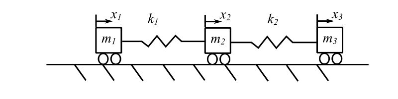
![\begin{equation*}[m]=\begin{bmatrix}m_1 & 0 & 0 \\0 & m_2 & 0 \\0 & 0 & m_3 \\\end{bmatrix}\end{equation*}](https://engcourses-uofa.ca/wp-content/ql-cache/quicklatex.com-9b12243663d135c70ed2f7ab57d46beb_l3.png "Rendered by QuickLaTeX.com")
![\begin{equation*}[k]=\begin{bmatrix}k_1 & -k_1 & 0 \\-k_1 & k_1+ k_2 & -k_2 \\0 & -k_2 & k_2 \\\end{bmatrix}\end{equation*}](https://engcourses-uofa.ca/wp-content/ql-cache/quicklatex.com-6928e0ee7372be20d807a5960f1f9db2_l3.png "Rendered by QuickLaTeX.com")
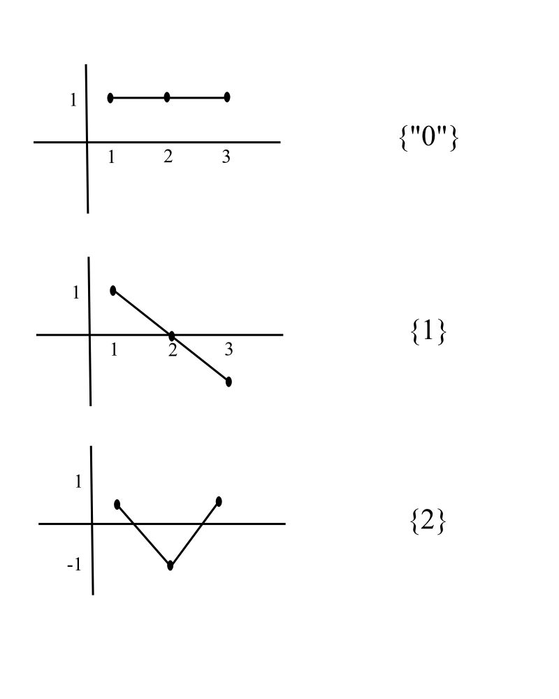
but the stiffness matrix is not positive definitive. It is singular. This is because one “natural frequency” is zero.
![\[p_o = 0\]](https://engcourses-uofa.ca/wp-content/ql-cache/quicklatex.com-5f60566c0ce7b00cb69ac651b2b80589_l3.png "Rendered by QuickLaTeX.com")

 is called a zeroth mode
![\begin{equation*} [k] \{u\}= \begin{bmatrix} k_1 & -k_1 & 0 \\ -k_1 & k_1+ k_2 & -k_2 \\ 0 & -k_2 & k_2 \\ \end{bmatrix} \begin{bmatrix} 1\\ 1\\ 1\\ \end{bmatrix} = \begin{bmatrix} 0\\ 0\\ 0\\ \end{bmatrix} =\{u\}^{T}[k] \end{equation*}](https://engcourses-uofa.ca/wp-content/ql-cache/quicklatex.com-3ef5196621616e2658406df5cec37418_l3.png "Rendered by QuickLaTeX.com")
Therefore
![\begin{equation*}\{u\}^{T}[m]\begin{Bmatrix}\ddot{x}_1\\\ddot{x}_2\\\ddot{x}_3\\\end{Bmatrix}=0\end{equation*}](https://engcourses-uofa.ca/wp-content/ql-cache/quicklatex.com-1de668bf4449e7ceab0765ed1a66aa6e_l3.png "Rendered by QuickLaTeX.com")
but since ![[m]](https://engcourses-uofa.ca/wp-content/ql-cache/quicklatex.com-04fd13cfffa1864cf42c2e3f94f29dcb_l3.png "Rendered by QuickLaTeX.com") is positive definite
is positive definite ![\{u\}^{T}[m] \neq 0](https://engcourses-uofa.ca/wp-content/ql-cache/quicklatex.com-92556771098bdc2866853970ef7d5723_l3.png "Rendered by QuickLaTeX.com") , therefore
, therefore  ,
, 
and the system is simply moving off in one direction. To suppress this mode we set:
![\[\{u_o\}^{T}[m]\{x\}= 0\]](https://engcourses-uofa.ca/wp-content/ql-cache/quicklatex.com-833ba34d757612644274b04dbc290051_l3.png "Rendered by QuickLaTeX.com")
This is the constraint equation:

![\[m_1 x_1 + m_2 x_2 + m_3 x_3 = 0\]](https://engcourses-uofa.ca/wp-content/ql-cache/quicklatex.com-da5b71315fc6c1b8004285122bba8ee8_l3.png "Rendered by QuickLaTeX.com")
or
![\[m_1 \dot{x}_1 + m_2 \dot{x}_2 + m_3 \dot{x}_3 = 0\]](https://engcourses-uofa.ca/wp-content/ql-cache/quicklatex.com-32c5aea8fbef10ab407bd4c0ce95ee2b_l3.png "Rendered by QuickLaTeX.com")
Where this expression says the momentum of the 3 masses must be zero. This essentially says this is a 2 DOF system.
Note: If we tried to find a flexibility matrix it is not defined.
We can write the constraint in a compound form as:
![\begin{equation*}\begin{Bmatrix}x_1\\x_2\\x_3\\\end{Bmatrix}=\begin{bmatrix}1 & 0 & 0 \\0 & 1 & 0 \\\frac{-m_1}{m_3} & \frac{-m_2}{m_3} & 0 \\\end{bmatrix}\begin{Bmatrix}x_1\\x_2\\x_3\\\end{Bmatrix}=\begin{bmatrix}1 & 0 \\0 & 1 \\\frac{-m_1}{m_3} & \frac{-m_2}{m_3} \\\end{bmatrix}\begin{Bmatrix}x_1\\x_2\\\end{Bmatrix}=[C]\begin{Bmatrix}x_1\\x_2\\\end{Bmatrix}\end{equation*}](https://engcourses-uofa.ca/wp-content/ql-cache/quicklatex.com-fad8a549a29c28edff8da1ee224b6e2c_l3.png "Rendered by QuickLaTeX.com")
We can now solve the eigenvalue problem using
![\[ [k^{'}] = [C]^{T}[k][C] \]](https://engcourses-uofa.ca/wp-content/ql-cache/quicklatex.com-48d1d1c514689b66835a1e0c59317ff4_l3.png "Rendered by QuickLaTeX.com")
![\[ [m^{'}] = [C]^{T}[m][C] \]](https://engcourses-uofa.ca/wp-content/ql-cache/quicklatex.com-c107d6c592077e2fe52ba1e90f0d4a12_l3.png "Rendered by QuickLaTeX.com")
so that
![\[ [k^{'}]\{u\} = p^{2}[m^{'}]\{u\} \]](https://engcourses-uofa.ca/wp-content/ql-cache/quicklatex.com-bbb382ac5b8c366a96170511c49cbe13_l3.png "Rendered by QuickLaTeX.com")
For the example above set  ,
, 
![\begin{equation*}[k']=\begin{bmatrix}1 & 0 & -1 \\0 & 1 & -1 \\\end{bmatrix}\begin{bmatrix}k & -k & 0 \\-k & 2k & -k \\0 & -k & k \\\end{bmatrix}\begin{bmatrix}1 & 0 \\0 & 1 \\-1 & -1 \\\end{bmatrix}=\begin{bmatrix}1 & 0 & -1 \\0 & 1 & -1 \\\end{bmatrix}\begin{bmatrix}k & -k \\0 & 3k \\-k & -2k \\\end{bmatrix}=\begin{bmatrix}2k & k \\k & 5k \\\end{bmatrix}\end{equation*}](https://engcourses-uofa.ca/wp-content/ql-cache/quicklatex.com-612607e7fdea73e1081758218ca6ffb8_l3.png "Rendered by QuickLaTeX.com")
![\begin{equation*}[m'] = m\begin{bmatrix}2 & 1 \\1 & 2 \\\end{bmatrix}\end{equation*}](https://engcourses-uofa.ca/wp-content/ql-cache/quicklatex.com-a8bbf07c128053db2ad0b217013ff6e9_l3.png "Rendered by QuickLaTeX.com")


![\[\left(2-2\frac{p^{2}m}{k}\right)\left(5-2\frac{p^{2}m}{k}\right) - \left(1 - \frac{p^{2}m}{k}\right)^{2} = 0\]](https://engcourses-uofa.ca/wp-content/ql-cache/quicklatex.com-980c5f50669799042d007762aa61019c_l3.png "Rendered by QuickLaTeX.com")
![\[10-14\frac{p^{2}m}{k} + 4\left(\frac{p^{2}m}{k}\right)^{2} - [1 - 2\frac{p^{2}m}{k} + \frac{p^{4}m^{2}}{k^{2}}] = 0 \]](https://engcourses-uofa.ca/wp-content/ql-cache/quicklatex.com-73ff8aabea89dd592ac2eaf711b55181_l3.png "Rendered by QuickLaTeX.com")
![\[9 - 12 \frac{p^{2}m}{k} + 3 \frac{p^{4}m^{2}}{k^{2}} = 0\]](https://engcourses-uofa.ca/wp-content/ql-cache/quicklatex.com-c2ca5391514ab116c58aa744a96ece26_l3.png "Rendered by QuickLaTeX.com")
![\[\frac{p^{4}m^{2}}{k^{2}} - \frac{4p^{2}m}{k} + 3 = 0\]](https://engcourses-uofa.ca/wp-content/ql-cache/quicklatex.com-36cd512b5902243fff327dd0a1bc1828_l3.png "Rendered by QuickLaTeX.com")
![\[p^{2} = \{2 \pm \sqrt{1}\} \frac{k}{m}\]](https://engcourses-uofa.ca/wp-content/ql-cache/quicklatex.com-0e17de85322401d5452df28ebf0a822a_l3.png "Rendered by QuickLaTeX.com")
![\[p^{2}_{1,2} = \frac{k}{m}, \frac{3k}{m}\]](https://engcourses-uofa.ca/wp-content/ql-cache/quicklatex.com-78b36150638c2cddaceb8d3367f48977_l3.png "Rendered by QuickLaTeX.com")


![\[x_3 = -x_1 - x_2\]](https://engcourses-uofa.ca/wp-content/ql-cache/quicklatex.com-7348f79dd58ae87fd06b577359182038_l3.png "Rendered by QuickLaTeX.com")


A second example of a 2DOF system is the vibration absorber as it can provide quite spectacular results when applied correctly. We will consider it first as a 2DOF undamped system, then include viscous damping. The closed form solution for the case of damping is much more involved.
Undamped Vibration Absorber
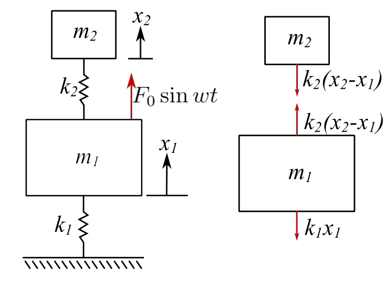
![\[\begin{split} + \uparrow \sum F_{x_1} &= m_1 \ddot{x_1} \\&= -k_1x_1 + k_2(x_2 - x_1) + F_o\sin\omega t \quad (1) \end{split} \]](https://engcourses-uofa.ca/wp-content/ql-cache/quicklatex.com-d01c084202be78d8a14b09ee716ddc0e_l3.png "Rendered by QuickLaTeX.com")
![\[ \begin{split} + \uparrow \sum F_{x_2} &= m_2\ddot{x_2} \\&= -k_2(x_2 - x_1) \quad (2) \end{split} \]](https://engcourses-uofa.ca/wp-content/ql-cache/quicklatex.com-3abd8278952ac20844621a596f60cfd5_l3.png "Rendered by QuickLaTeX.com")
![\[ m_1\ddot{x_1} + (k_1+k_2)x_1 - k_2x_2 = F_o \sin\omega t \]](https://engcourses-uofa.ca/wp-content/ql-cache/quicklatex.com-ebe34c2e4b80fdfa43eb579fcc783136_l3.png "Rendered by QuickLaTeX.com")
![\[ m_2\ddot{x_2} - k_2x_1 + k_2x_2 = 0 \]](https://engcourses-uofa.ca/wp-content/ql-cache/quicklatex.com-cec5f376de15940c836f656266bfede4_l3.png "Rendered by QuickLaTeX.com")
![\[ \begin{bmatrix} m_1 & 0 \\ 0 & m_2 \end{bmatrix} \begin{Bmatrix} \ddot{x_1} \\ \ddot{x_2} \end{Bmatrix} + \begin{bmatrix} k_1+k_2 & -k_2 \\ -k_2 & k_2 \end{bmatrix} \begin{Bmatrix} x_1 \\ x_2 \end{Bmatrix} = \begin{Bmatrix} F_o\sin\omega t \\ 0 \end{Bmatrix} \]](https://engcourses-uofa.ca/wp-content/ql-cache/quicklatex.com-f4046f37f62d94249c27bb4f6e0ccf4b_l3.png "Rendered by QuickLaTeX.com")
For S.S. solution, assume:
![\[\begin{Bmatrix} x_1 \\ x_2 \end{Bmatrix} = \begin{Bmatrix} X_1 \\ X_2 \end{Bmatrix} \sin \omega t \]](https://engcourses-uofa.ca/wp-content/ql-cache/quicklatex.com-e6dbf39b66fe52adc7be291d18256db8_l3.png "Rendered by QuickLaTeX.com")
Under the steady state assumption, the equations of motion become:
![\[ [-m_1\omega^2 + k_1 + k_2]X_1 - k_2X_2 = F_o \quad (*) \]](https://engcourses-uofa.ca/wp-content/ql-cache/quicklatex.com-7865265fc8e04ff6893fb57160af7afe_l3.png "Rendered by QuickLaTeX.com")
![\[-k_2X_1 + (k_2 - m_2\omega^2)X_2 = 0 \quad (**) \]](https://engcourses-uofa.ca/wp-content/ql-cache/quicklatex.com-51f7f6ba9912e722d367c4c0645a910c_l3.png "Rendered by QuickLaTeX.com")
Therefore, from  :
:
![\[ X_2 = \frac{k_2X_1}{(k_2-m_2\omega^2)}\]](https://engcourses-uofa.ca/wp-content/ql-cache/quicklatex.com-53ebd64eeb209eedebd37f14e031fa2c_l3.png "Rendered by QuickLaTeX.com")
And then from  :
:
![\[(k_1 +k_2-m_1\omega^2)X_1 - \frac{k_2^2X_1}{k_2-m_2\omega^2} = F_o\]](https://engcourses-uofa.ca/wp-content/ql-cache/quicklatex.com-ce1e42abd912bfd5985c0ef36d6c1c56_l3.png "Rendered by QuickLaTeX.com")
-k_2^2\Big\}X_1}{k_2-m_2\omega^2} = F_o \]](https://engcourses-uofa.ca/wp-content/ql-cache/quicklatex.com-60d75cde7c2841c3ec388b835f9984ee_l3.png "Rendered by QuickLaTeX.com")
Therefore:
![\[X_1 = \frac{F_o(k_2-m_2\omega^2)}{[(k_2-m_2\omega^2)(k_1+k_2-m_1\omega^2) - k_2^2]} \]](https://engcourses-uofa.ca/wp-content/ql-cache/quicklatex.com-d64fff0a7b738f411a39a1e9782dfbf8_l3.png "Rendered by QuickLaTeX.com")
![\[X_2 = \frac{k_2F_o}{[(k_2 - m_2\omega^2)(k_1+k_2-m_1\omega^2)-k_2^2]} \]](https://engcourses-uofa.ca/wp-content/ql-cache/quicklatex.com-2d4481cdafbba6a945919c584455a492_l3.png "Rendered by QuickLaTeX.com")
For use in vibration absorber applications, we define:
![\[p_{11} := \sqrt{\frac{k_1}{m_1}},\ p_{22} := \sqrt{\frac{k_2}{m_2}},\ \mu := \frac{m_2}{m_1} \]](https://engcourses-uofa.ca/wp-content/ql-cache/quicklatex.com-fe6b6ea541f974f00632167bc00d91d5_l3.png "Rendered by QuickLaTeX.com")
Then divide numerator and denominator by  .
.
For the 2DOF system shown with the forcing appiled to the mass  , the response of the masses and
  is:
is:
![\[X_1 = \frac{F_o(k_2-m_2\omega^2)}{(k_2-m_2\omega^2)(k_1+k_2-m_1\omega^2)-k_2^2} \quad (*) \]](https://engcourses-uofa.ca/wp-content/ql-cache/quicklatex.com-9a09cba3496f89448d2c4d1ffc3af0b6_l3.png "Rendered by QuickLaTeX.com")
![\[X_2 = \frac{F_ok_2}{(k_2-m_2\omega^2)(k_1+k_2-m_1\omega^2)-k_2^2} \quad (**) \]](https://engcourses-uofa.ca/wp-content/ql-cache/quicklatex.com-6ca2176826a3d17a06cabbb725037fd5_l3.png "Rendered by QuickLaTeX.com")
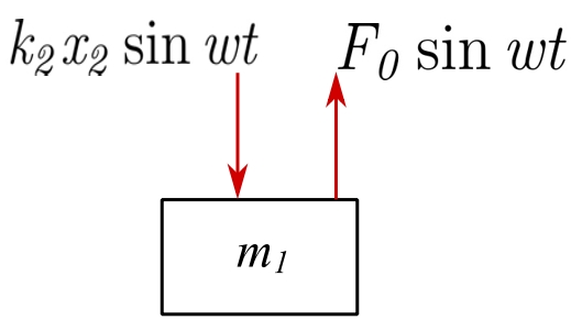
It is seen that from that if  or
or  , then the mass is stationary. This leads to the idea that the motion of can theoretically be reduced to zero if we employ , at the operating frequency
  . For this application. the subsystem , is called a vibration absorber and at the operating frequency:
![\[X_1 = 0 \text{ and } X_2 = \frac{-F_o}{k_2} \]](https://engcourses-uofa.ca/wp-content/ql-cache/quicklatex.com-d6c3ebc28106091c9cec9c6b239e7ef9_l3.png "Rendered by QuickLaTeX.com")
For this application it is useful to modify and to reflect what we can call – the original system , , the absorber system , using the definitions:
Using those definitions show that and become:
![\[X_1 = \frac{\frac{F_o}{k_1}\left[1-\left(\frac{\omega}{p_{22}}\right)^2\right]}{\left{\left[1-\left(\frac{\omega}{p_{22}}\right)^2\right]\left[1+\mu\left(\frac{p_{22}}{p_{11}}\right)^2-\left(\frac{\omega^2}{p_{11}}\right)^2\right] - \mu\left(\frac{p_{22}}{p_{11}}\right)^2\right}} \]](https://engcourses-uofa.ca/wp-content/ql-cache/quicklatex.com-3560b0bf3b50cdb0e152881b5ae2f268_l3.png "Rendered by QuickLaTeX.com")
![\[X_2 = \frac{\frac{F_o}{k_1}}{\left{\left[1-\left(\frac{\omega}{p_{22}}\right)^2\right]\left[1+\mu\left(\frac{p_{22}}{p_{11}}\right)^2-\left(\frac{\omega^2}{p_{11}}\right)^2\right] - \mu\left(\frac{p_{22}}{p_{11}}\right)^2\right}} \]](https://engcourses-uofa.ca/wp-content/ql-cache/quicklatex.com-895105d702afd5915b7c63c213c3359e_l3.png "Rendered by QuickLaTeX.com")
And when  :
:
![\[X_1 = 0,\ X_2 = -\frac{F_o}{k_2}\]](https://engcourses-uofa.ca/wp-content/ql-cache/quicklatex.com-d565825a50fea752d4449bdaf27bfd93_l3.png "Rendered by QuickLaTeX.com")
This shows that when the subsystem , is timed so  that is motionless as the force in the spring exactly opposes the excitation force
  .
.
The natural frequencies of the combined system are found from setting the denominator of the responses  ,
,  to zero. Therefore, the natural frequencies are found when is replaced by
  and the expression becomes:
![\[ \Big[1 - \Big(\frac{p}{p_{22}}\Big)^2\Big]\Big[1 + \mu\Big(\frac{p_{22}}{p_{11}}\Big)^2-\Big(\frac{p}{p_{11}}\Big)^2\Big] - \mu\Big(\frac{p_{22}}{p_{11}}\Big)^2 = 0\]](https://engcourses-uofa.ca/wp-content/ql-cache/quicklatex.com-3390c9036e36548617d6fda53e79db7d_l3.png "Rendered by QuickLaTeX.com")
![\[1 + \mu\Big(\frac{p_{22}}{p_{11}}\Big)^2-\Big(\frac{p}{p_{11}}\Big)^2-\Big(\frac{p}{p_{22}}\Big)^2-\mu\Big(\frac{p_{22}}{p_{11}}\Big)^2\Big(\frac{p}{p_{22}}\Big)^2+\Big(\frac{p}{p_{11}}\Big)^2\Big(\frac{p}{p_{22}}\Big)^2 -\mu\Big(\frac{p_{22}}{p_{11}}\Big)^2 = 0\]](https://engcourses-uofa.ca/wp-content/ql-cache/quicklatex.com-6825f7c2da835e63687cbca5ce71e210_l3.png "Rendered by QuickLaTeX.com")
Therefore:
![\[\Big(\frac{p}{p_{22}}\Big)^4\Big(\frac{p_{22}}{p_{11}}\Big)^2-\Big(\frac{p}{p_{22}}\Big)^2\Big[1+\mu\Big(\frac{p_{22}}{p_{11}}\Big)^2 + \Big(\frac{p_{22}}{p_{11}}\Big)^2\Big] + 1= 0 \]](https://engcourses-uofa.ca/wp-content/ql-cache/quicklatex.com-063b598d0a615285c87d1fc5b34b7c02_l3.png "Rendered by QuickLaTeX.com")
![\[\Big(\frac{p}{p_{22}}\Big)^4-\Big(\frac{p}{p_{22}}\Big)^2\Big[1+\mu+\Big(\frac{p_{11}}{p_{22}}\Big)^2\Big] + \Big(\frac{p_{11}}{p_{22}}\Big)^2 = 0 \quad (*) \]](https://engcourses-uofa.ca/wp-content/ql-cache/quicklatex.com-0bd4d50bb97ef6888c3a64dcf9ec5224_l3.png "Rendered by QuickLaTeX.com")
If  , this becomes:
![\[\Big(\frac{p}{p_{22}}\Big)^4 - \Big(\frac{p}{p_{22}}\Big)^2[2+\mu] + 1 = 0\]](https://engcourses-uofa.ca/wp-content/ql-cache/quicklatex.com-dc26b38298f81c44cf415098578f8e17_l3.png "Rendered by QuickLaTeX.com")
If instead of the mass being excited by the force  , the exication is through the base as
  , what is the difference in the response of and of masses and ?
The mass ratio,  , essentially determines the spread of the two resonances:
![\[\mu = 0.1, \quad \frac{\omega}{p_{22}} = 0.85,\ 1.17\]](https://engcourses-uofa.ca/wp-content/ql-cache/quicklatex.com-12152ea5054d190a67c4a12623d44172_l3.png "Rendered by QuickLaTeX.com")
![\[\mu = 0.2, \quad \frac{\omega}{p_{22}} = 0.79,\ 1.25\]](https://engcourses-uofa.ca/wp-content/ql-cache/quicklatex.com-4ac2dec6bf7c51dd4c6a877e9371738c_l3.png "Rendered by QuickLaTeX.com")
![\[\mu = 0.05, \quad \frac{\omega}{p_{22}} = 0.89,\ 1.122\]](https://engcourses-uofa.ca/wp-content/ql-cache/quicklatex.com-e49514953ac4d8f9ffc38280fdf2a933_l3.png "Rendered by QuickLaTeX.com")
( )
)
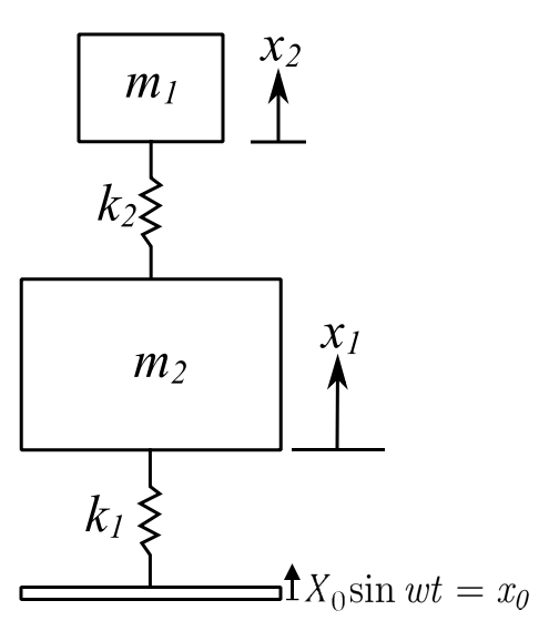
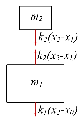
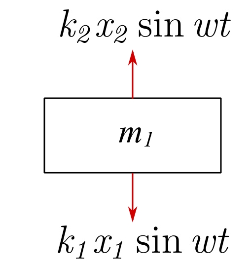
![\[\begin{split} \sum F_{x_1} &= m_1\ddot{x_1} \\&= -k_1(x_1-x_o) + k_2(x_2-x_1) \quad (1) \end{split} \]](https://engcourses-uofa.ca/wp-content/ql-cache/quicklatex.com-d8d9fa90d1a36c9bc748e7cdeca82f72_l3.png "Rendered by QuickLaTeX.com")
![\[\begin{split} \sum F_{x_2} &= m_2\ddot{x_2} \\&=-k_2(x_2-x_1) \quad (2) \end{split}\]](https://engcourses-uofa.ca/wp-content/ql-cache/quicklatex.com-188f3a4150550245ca364ba5b74b3415_l3.png "Rendered by QuickLaTeX.com")
Therefore, the equations are identical except that is replaced by  . The response of
  and
and  for the vibration absorber is:
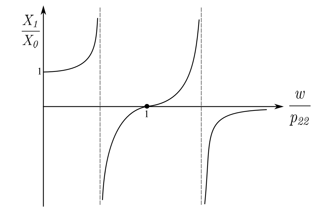
![\[X_1= \frac{X_0[1-(\frac{\omega}{p_{22}})^2]}{\{[1-(\frac{\omega}{p_{22}})^2][1+\mu(\frac{p_{22}}{p_{11}})^2-(\frac{\omega}{p_{11}})^2]-\mu(\frac{p_{22}}{p_{11}})^2\}}\]](https://engcourses-uofa.ca/wp-content/ql-cache/quicklatex.com-ad377993fb6b9b7ff03f81bd9abbca4b_l3.png "Rendered by QuickLaTeX.com")
![\[X_2= \frac{X_0}{\{[1-(\frac{\omega}{p_{22}})^2][1+\mu(\frac{p_{22}}{p_{11}})^2-(\frac{\omega}{p_{11}})^2]-\mu(\frac{p_{22}}{p_{11}})^2\}}\]](https://engcourses-uofa.ca/wp-content/ql-cache/quicklatex.com-1308f34271d455f805a1d6b6c7c50e58_l3.png "Rendered by QuickLaTeX.com")
Again when  :
:
![\[X_1 = 0\]](https://engcourses-uofa.ca/wp-content/ql-cache/quicklatex.com-690cfc2b55e0bd2d7cbf72725dd304af_l3.png "Rendered by QuickLaTeX.com")
![\[\begin{split} X_2 &= -X_o\frac{1}{\mu}\Big(\frac{p_{11}}{p_{22}}\Big)^2 \\&= -X_o\frac{m_1}{m_2}\frac{k_1}{m_1}\frac{m_2}{k_2} \\&= -X_o\frac{k_1}{k_2} \end{split} \]](https://engcourses-uofa.ca/wp-content/ql-cache/quicklatex.com-9963cf284867a8ccf0bb8f826b73a76e_l3.png "Rendered by QuickLaTeX.com")
Therefore,  so that at any time:
And the net dynamic force on is zero!
To solve the system with damping it is more advantageous to use complex numbers:
![\[\{x\} =\{X\}e^{i\omega t}\]](https://engcourses-uofa.ca/wp-content/ql-cache/quicklatex.com-18a4a26825ff7baf5c8e1cebc3d10d59_l3.png "Rendered by QuickLaTeX.com")
Or:
![\[\{x\} =\{\zeta\}e^{st}\]](https://engcourses-uofa.ca/wp-content/ql-cache/quicklatex.com-b40abf0bcff1432d5211f878ba162086_l3.png "Rendered by QuickLaTeX.com")
There are a number of special cases of the general forced damped analysis that are useful.
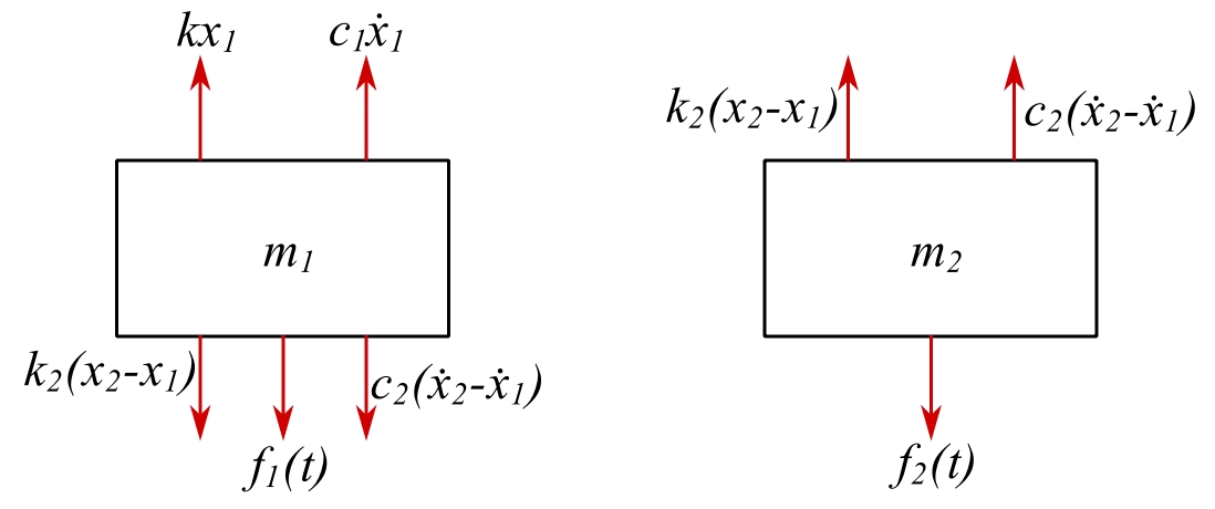
Damped Forced 2DOF System
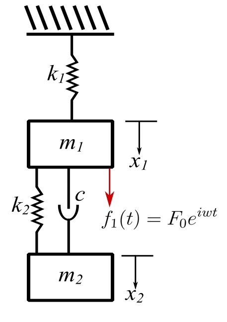
Consider a general damped system that can be specialized for special applications.
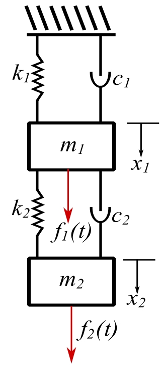
![\[f_1(t) = f_1e^{st}\]](https://engcourses-uofa.ca/wp-content/ql-cache/quicklatex.com-5c8ace2d5553025207ae87466a10174f_l3.png "Rendered by QuickLaTeX.com")
![\[f_2(t) = f_2e^{st}\]](https://engcourses-uofa.ca/wp-content/ql-cache/quicklatex.com-2f493534998c0be0e96021c8717ca34c_l3.png "Rendered by QuickLaTeX.com")
![\[m\ddot{x_1} = k_2(x_2 - x_1) + c_2(\dot{x_2}-\dot{x_1}) - k_1x_1 - c_1\dot{x_1} + f_1(t) \]](https://engcourses-uofa.ca/wp-content/ql-cache/quicklatex.com-ad11001555f932290dcce2eeebe0712e_l3.png "Rendered by QuickLaTeX.com")
![\[m\ddot{x_1} + (k_1+k_2)x_1 + (c_1+c_2)\dot{x_1} - k_2x_2 - c_2\dot{x_2} = f_1(t) \]](https://engcourses-uofa.ca/wp-content/ql-cache/quicklatex.com-41240edda03157946b6f1222a90d5a11_l3.png "Rendered by QuickLaTeX.com")
![\[m_2\ddot{x_2} = f_2(t) - k_2(x_2-x_1)-c_2(\dot{x_2}-\dot{x_1})\]](https://engcourses-uofa.ca/wp-content/ql-cache/quicklatex.com-fbf32f987baf28647c21d86fe83e9e4a_l3.png "Rendered by QuickLaTeX.com")
Assume a solution
![\[\begin{Bmatrix} x_1 \\ x_2 \end{Bmatrix} = \begin{Bmatrix} \zeta_1 \\ \zeta_2 \end{Bmatrix} e^{st}\]](https://engcourses-uofa.ca/wp-content/ql-cache/quicklatex.com-19b3d3a0d13ced78a662c3588bcb1b05_l3.png "Rendered by QuickLaTeX.com")
Thus:
![\[[m_1s^2 + (c_1+c_2)s + (k_1+k_2)]\zeta_1 - [c_2s+k_2]\zeta_2 = f_1\]](https://engcourses-uofa.ca/wp-content/ql-cache/quicklatex.com-1a6f0c0e5ad028b843eeb5e32b734af4_l3.png "Rendered by QuickLaTeX.com")
![\[-(c_2s + k_2)\zeta_1 + [m_2s^2+c_2s+k_2]\zeta_2 = f_2\]](https://engcourses-uofa.ca/wp-content/ql-cache/quicklatex.com-5a42471cfc8139c3efddc17041048e3d_l3.png "Rendered by QuickLaTeX.com")
Therefore:
![\[V_{11} = m_1s^2 + (c_1 + c_2)s + k_1 + k_2 \]](https://engcourses-uofa.ca/wp-content/ql-cache/quicklatex.com-dd0259bcd62a54af36e2d0ae6ca00efc_l3.png "Rendered by QuickLaTeX.com")
![\[V_{12} = -(c_2s + k_2) = V_{21} \]](https://engcourses-uofa.ca/wp-content/ql-cache/quicklatex.com-3b64eda3b37bacc4ef4c4192683b9d95_l3.png "Rendered by QuickLaTeX.com")
![\[V_{22} = m_2s^2 + c_2s + k_2 \]](https://engcourses-uofa.ca/wp-content/ql-cache/quicklatex.com-3838ab0e50a794e52dd5b2f7895b2602_l3.png "Rendered by QuickLaTeX.com")
![\[V_{11}\zeta_1 + V_{12}\zeta_2 = f_1\]](https://engcourses-uofa.ca/wp-content/ql-cache/quicklatex.com-83e313289e264d8c446757b6c9768091_l3.png "Rendered by QuickLaTeX.com")
![\[V_{21}\zeta_1 + V_{22}\zeta_2 = f_2\]](https://engcourses-uofa.ca/wp-content/ql-cache/quicklatex.com-9494c190210e22e843744abc6872b91c_l3.png "Rendered by QuickLaTeX.com")
And we wish to find  and
and  :
:
![\[ \begin{bmatrix} V_11 & V_12 \\ V_21 & V_22 \end{bmatrix} \begin{bmatrix} \zeta_1 \\ \zeta_2 \end{bmatrix} = \begin{bmatrix} f_1 \\ f_2 \end{bmatrix} \]](https://engcourses-uofa.ca/wp-content/ql-cache/quicklatex.com-6cc75c89afb4457466a3864d90178026_l3.png "Rendered by QuickLaTeX.com")
![\[ [V]^{-1} \equiv [Y] \]](https://engcourses-uofa.ca/wp-content/ql-cache/quicklatex.com-99c342ce407794d1b6d440b5686ac5cd_l3.png "Rendered by QuickLaTeX.com")
![\[Y_{11}(s) = \frac{V_{22}(s)}{\Delta},\ Y_{12} = -\frac{V_{21}(s)}{\Delta},\ Y_{22} = \frac{V_{11}(s)}{\Delta}\]](https://engcourses-uofa.ca/wp-content/ql-cache/quicklatex.com-c06b840cc4be1c23d640fd14f01a285c_l3.png "Rendered by QuickLaTeX.com")
Where  . Thus:
![\[\zeta_1 = Y_{11}(s)f_1 + Y_{12}(s)f_2\]](https://engcourses-uofa.ca/wp-content/ql-cache/quicklatex.com-b8f0d104835075d1533db2f2b403bd1b_l3.png "Rendered by QuickLaTeX.com")
![\[\zeta_2 = Y_{21}(s)f_1 + Y_{22}(s)f_2\]](https://engcourses-uofa.ca/wp-content/ql-cache/quicklatex.com-6cdadf81c3b26ad50837b3d36fdfc399_l3.png "Rendered by QuickLaTeX.com")
There is a lot hidden in these symbols so we can consider some special cases.
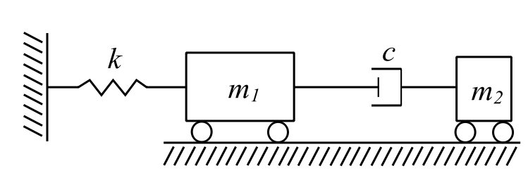
1. Untuned Viscous Vibration Absorber
(Houdaille damper or viscous Lanchester damper)
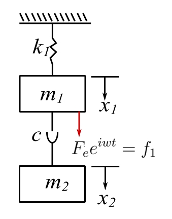
If we look at our general solution then:
![\[c_2 = c,\ c_1 = 0,\ k_2 = 0,\ f_2 = 0 \]](https://engcourses-uofa.ca/wp-content/ql-cache/quicklatex.com-c3255670deef5417c7a00d92d6fac5aa_l3.png "Rendered by QuickLaTeX.com")
![\[V_{11} = m_1s^2 + cs + k_1 \]](https://engcourses-uofa.ca/wp-content/ql-cache/quicklatex.com-d95b60295b0a284cab3be9ba9d4567fa_l3.png "Rendered by QuickLaTeX.com")
![\[V_{12} = -cs = V_{21} \]](https://engcourses-uofa.ca/wp-content/ql-cache/quicklatex.com-3ae174963d08416d622bdf65bfbb79b2_l3.png "Rendered by QuickLaTeX.com")
![\[V_{22} = m_2s^2 + cs \]](https://engcourses-uofa.ca/wp-content/ql-cache/quicklatex.com-bcb7ea18b6708a1c8d7bb6ded944c8c7_l3.png "Rendered by QuickLaTeX.com")
![\[\zeta_1 = Y_{11}(s) f_1,\quad Y_{11}(s) = \frac{V_{22}(s)}{\Delta} \]](https://engcourses-uofa.ca/wp-content/ql-cache/quicklatex.com-3092e8d78e02bacf56f8122a6b026653_l3.png "Rendered by QuickLaTeX.com")
![\[\zeta_2 = Y_{21}(s) f_1,\quad Y_{21}(s) = -\frac{V_{21}(s)}{\Delta} \]](https://engcourses-uofa.ca/wp-content/ql-cache/quicklatex.com-587e77f24afb91b98277f4db805dfe11_l3.png "Rendered by QuickLaTeX.com")
Therefore:
![\[ \Delta = [m_1s^2 + cs + k][m_2s^2 + cs] - (cs)^2 \]](https://engcourses-uofa.ca/wp-content/ql-cache/quicklatex.com-bc1551ac04edbd7b5312e99e180993a4_l3.png "Rendered by QuickLaTeX.com")
Put  :
:
![\[\begin{split} \Delta &= [k-m_1\omega^2 + ic\omega][-m_2\omega^2 +ic\omega]+c^2\omega^2 \\&= -m_2\omega^2(k-m_1\omega^2) + ic\omega[-m_2\omega^2 + (k-m\omega^2) \end{split} \]](https://engcourses-uofa.ca/wp-content/ql-cache/quicklatex.com-11a893617ce60b473f3fc4c1027226bf_l3.png "Rendered by QuickLaTeX.com")
Therefore:
![\[ \zeta_1 = \frac{(-m_2\omega^2 + ic\omega)F_o}{-m_2\omega^2(k-m_1\omega^2) +ic\omega[-m_2\omega^2 + (k-m\omega^2)]}\]](https://engcourses-uofa.ca/wp-content/ql-cache/quicklatex.com-d58fd8a76e1b0754838df1f4cf47a05f_l3.png "Rendered by QuickLaTeX.com")
![\[ \zeta_2 = \frac{ic\omega}{-m_2\omega^2(k-m_1\omega^2) + ic\omega[-m_2\omega^2 + (k-m\omega^2)]} \]](https://engcourses-uofa.ca/wp-content/ql-cache/quicklatex.com-cf541baac4efb865a82fe44c746fb654_l3.png "Rendered by QuickLaTeX.com")
We are really interested in the amplitudes. Use the result that if:
![\[\begin{split} \zeta &= \frac{B+iC}{D+iE} \cdot \frac{D-iE}{D-iE} \\&=\frac{BD+CE+i(CD-BE)}{D^2+E^2} \end{split} \]](https://engcourses-uofa.ca/wp-content/ql-cache/quicklatex.com-f47e78813f09a37aea146736b3d0cb11_l3.png "Rendered by QuickLaTeX.com")
We wish to write  .
.
![\[ \begin{split} A &= \frac{\sqrt{(BD+CE)^2 + (CD-BE)^2}}{D^2 + E^2} \\&= \frac{\sqrt{(BD)^2 + (CE)^2 + 2BDCE + (CD)^2 + (BE)^2 - 2BCDE}}{D^2+E^2} \\&= \frac{\sqrt{B^2(D^2+E^2) + C^2(D^2+E^2)}}{D^2+E^2} \\&= \sqrt{\frac{B^2+C^2}{D^2+E^2}} \end{split} \]](https://engcourses-uofa.ca/wp-content/ql-cache/quicklatex.com-46b910ff63a11c35cf3a097681cc3598_l3.png "Rendered by QuickLaTeX.com")
![\[ \alpha = \tan^{-1} \frac{CD-BE}{BD+CE} \]](https://engcourses-uofa.ca/wp-content/ql-cache/quicklatex.com-1e907fddf1e6cc7876228f932a8996d4_l3.png "Rendered by QuickLaTeX.com")
![\[X_1 = \frac{F_o\sqrt{(m_2\omega^2)^2+(c\omega)^2}}{\sqrt{[m_2\omega^2(k-m_1\omega^2)]^2+(c\omega)^2[m_2\omega^2 - (k-m_1\omega^2)]^2}} \]](https://engcourses-uofa.ca/wp-content/ql-cache/quicklatex.com-7ed245e0dff03639c9eb474e4d8454d1_l3.png "Rendered by QuickLaTeX.com")
![\[X_o = \frac{F_o}{k},\ p_1^2 = \frac{k_1}{m_1},\ \nu = \frac{c}{2m_1p_1},\ \mu = \frac{m_2}{m_1},\ r = \frac{\omega}{p_1} \]](https://engcourses-uofa.ca/wp-content/ql-cache/quicklatex.com-74a07f9ebfe11bc79ef5e308b0645db9_l3.png "Rendered by QuickLaTeX.com")
Thus:
![\[ \frac{X_1}{X_o} = \frac{\sqrt{(\frac{m_2}{k}\omega^2)^2 + (\frac{c\omega}{k})^2}}{\sqrt{[\frac{m_2\omega^2}{k}(1-\frac{m_1\omega^2}{k})]^2 + (\frac{c\omega}{k})^2[\frac{m_2\omega^2}{k} - (1- \frac{m_1\omega^2}{k})]^2}} \]](https://engcourses-uofa.ca/wp-content/ql-cache/quicklatex.com-496816ceea6a640cbd1f1114ad999ccc_l3.png "Rendered by QuickLaTeX.com")
![\[\frac{m_2}{m_1} \frac{m_1}{k} \omega^2 = \mu r^2 = \frac{m_2}{k}\omega^2\]](https://engcourses-uofa.ca/wp-content/ql-cache/quicklatex.com-52974e70ca04835de73d488eb81101ad_l3.png "Rendered by QuickLaTeX.com")
![\[\frac{c\omega}{k} = \frac{cm_1}{m_1k}\omega = \frac{c}{m_1p_1^2} \]](https://engcourses-uofa.ca/wp-content/ql-cache/quicklatex.com-4d5884f71c19ce744f7566c0e38f0ba3_l3.png "Rendered by QuickLaTeX.com")
![\[\omega = 2\nu r\]](https://engcourses-uofa.ca/wp-content/ql-cache/quicklatex.com-5535cac1f444f0b307f3369cf796e772_l3.png "Rendered by QuickLaTeX.com")
Thus:
![\[\begin{split} \frac{X_1}{X_o} &= \frac{\sqrt{\mu^2r^4 + (2\nu r)^2}}{\sqrt{[\mu r^2(1-r^2)]^2 + (2\nu r)^2[\mu r^2 - (1-r^2)]^2}} \\& = \frac{\sqrt{\mu^2r^2 + 4\nu ^2}}{\sqrt{[\mu r(1-r^2)]^2 + 4\nu ^2[\mu r^2 - (1-r^2)]^2}} \\&= \sqrt{\frac{N}{D}} \end{split} \]](https://engcourses-uofa.ca/wp-content/ql-cache/quicklatex.com-98c6a683033b268952ef45e81fad98e2_l3.png "Rendered by QuickLaTeX.com")
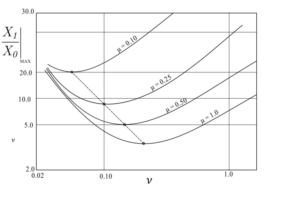
We wish to find the optimum ratio  which minimizes this amplitude;
![\[\begin{split} \frac{\text{d}\frac{X_1}{X_o}}{\text{d}\nu} &= \frac{D^{\frac{1}{2}}\frac{N^{-\frac{1}{2}}}{2}(8\nu) - N^{\frac{1}{2}}\frac{D^{\frac{-1}{2}}}{2}(8\nu)[\mu r^2 - (1-r^2)]^2}{D} \\&= 0 \end{split} \]](https://engcourses-uofa.ca/wp-content/ql-cache/quicklatex.com-5cee36945112a4f7f30656063ed4c275_l3.png "Rendered by QuickLaTeX.com")
Multiply by  . Therefore:
![\[ D-N[\mu r^2 - (1-r^2)]^2 = 0 \]](https://engcourses-uofa.ca/wp-content/ql-cache/quicklatex.com-ae1e0be0102944ca1ca14aef1d6630ea_l3.png "Rendered by QuickLaTeX.com")
![\[[\mu r(1-r^2)]^2 + 4\nu^2[\mu r^2 - (1-r^2)]^2 = (\mu^2 r^2 + 4\nu^2)[\mu r^2 - (1-r^2)]^2 \]](https://engcourses-uofa.ca/wp-content/ql-cache/quicklatex.com-908d02e95b1a20811b9a7d90647e5dbd_l3.png "Rendered by QuickLaTeX.com")
![\[[\mu r(1-r^2)]^2 = (\mu r)^2[\mu r^2 - (1-r^2)]^2 \]](https://engcourses-uofa.ca/wp-content/ql-cache/quicklatex.com-f5645eb5bca63a79d66f72e4fe4f46f6_l3.png "Rendered by QuickLaTeX.com")
![\[(1-r^2) = \mu r^2 - (1-r^2) \]](https://engcourses-uofa.ca/wp-content/ql-cache/quicklatex.com-a986d21d2932e5fb36af9652255dacef_l3.png "Rendered by QuickLaTeX.com")
![\[ 2(1-r^2) = \mu r^2 \]](https://engcourses-uofa.ca/wp-content/ql-cache/quicklatex.com-35f6672b15bcac4c9b8b2462f47fcbd6_l3.png "Rendered by QuickLaTeX.com")
![\[ 2 = r^2(2+\mu) \]](https://engcourses-uofa.ca/wp-content/ql-cache/quicklatex.com-9f3d65f6efd588e358e96d314e41df59_l3.png "Rendered by QuickLaTeX.com")
Therefore:
![\[r = \sqrt{\frac{2}{2+\mu}},\quad \mu = \frac{2(1-r^2)}{r^2} \]](https://engcourses-uofa.ca/wp-content/ql-cache/quicklatex.com-6b36d17525c16868d12187ac4b44aa72_l3.png "Rendered by QuickLaTeX.com")
Therefore, the minimum amplitude for optimum occurs when  . To find the value of , use this value of
  .
.
![\[ \begin{split} \frac{X_1}{X_o} &= \frac{\sqrt{\frac{\mu^2 2}{2+\mu} +4\nu^2}}{\sqrt{\frac{\mu^2 2}{2+\mu} (1- \frac{2}{2+\mu})^2 + 4\nu^2[\mu\frac{2}{2+\mu} - (1-\frac{2}{2+\mu})]^2}} \\&= \frac{\sqrt{\frac{2\mu^2}{2+\mu} + 4\nu^2}}{\sqrt{\frac{2\mu^2}{2+\mu}\frac{\mu^2}{(2+\mu)^2} + 4\nu^2[\frac{2\mu}{2+\mu} - (\frac{\mu}{2+\mu}) ]^2}} \\&= \frac{\sqrt{\frac{2\mu^2 + 4\nu(2+\mu)}{2+\mu}}}{\sqrt{\frac{2\mu^4}{(2+\mu)^3} + \frac{4\nu^2\mu^2}{(2+\mu)^2}}} \\&= \frac{\sqrt{2\mu^2 +4\nu^2(2+\mu)}}{\mu\sqrt{\frac{2\mu^2 + 4\nu^2(2+\mu)}{(2+\mu)^2}}} \\&= \frac{2+\mu}{\mu} = \frac{X_1}{X_o}\Big|_{\text{MAX}} \\&= 5\quad (\mu = \frac{1}{2}) \end{split} \]](https://engcourses-uofa.ca/wp-content/ql-cache/quicklatex.com-3fb39c0762df0d92a4f9d53d15c48b96_l3.png "Rendered by QuickLaTeX.com")
The amplitude at this value of is independent of !
![\[ \begin{split} \frac{X_1}{X_o} &= \frac{\sqrt{\mu^2r^2 + 4\nu^2}}{\sqrt{\mu^2r^2(1-2r^2+r^4)+4\nu^2[r^2(1+\mu)-1]^2}} \\&= \frac{\sqrt{\mu^2r^2 + 4\nu^2}}{\sqrt{\mu^2(r^2-2r^4+r^6) + 4\nu^2[r^4(1+\mu)^2-2r^2(1+\mu)+1]}} \\&= \sqrt{\frac{N}{D}} \end{split} \]](https://engcourses-uofa.ca/wp-content/ql-cache/quicklatex.com-005e385017dab6d2311e6d1ba92137a8_l3.png "Rendered by QuickLaTeX.com")
![\[ \begin{split} \frac{\text{d}(\frac{X_1}{X_o})}{\text{d}r} &= \frac{D^{\frac{1}{2}}\frac{N^{-\frac{1}{2}}}{2}2\mu^2r-N^{\frac{1}{2}}\frac{D^{-\frac{1}{2}}}{2}[\mu^2(2r+8r^3+6r^5) + 4\nu^2(4r^3(1+\mu)^2 - 4r(1+\mu))]}{D} \\& = 0 \end{split} \]](https://engcourses-uofa.ca/wp-content/ql-cache/quicklatex.com-47c13702f1f70ed325ca0922c6738090_l3.png "Rendered by QuickLaTeX.com")
Multiply by  . Then:
![\[ 0 = D(\mu^2r)-N[\mu^2(r-4r^3+3r^5) + 2\nu^2(4r^3(1+\mu)^2-4r(1+\mu))] \]](https://engcourses-uofa.ca/wp-content/ql-cache/quicklatex.com-a3dbd620edefd7094605f5c8efc68a96_l3.png "Rendered by QuickLaTeX.com")
Now evaluate this for  .
.
![\[D\mu^2 = N[\mu^2(1-4r^2+3r^4)+2\nu^2(4r^2(1+\mu)^2-4(1+\mu))] \]](https://engcourses-uofa.ca/wp-content/ql-cache/quicklatex.com-44ce7cb5abfb071bd99cac8d2be8b95c_l3.png "Rendered by QuickLaTeX.com")
Note that:
![\[ \begin{split} \frac{X_1}{X_0} &= \sqrt{\frac{N}{D}} \\&= \frac{2+\mu}{\mu} \end{split}\]](https://engcourses-uofa.ca/wp-content/ql-cache/quicklatex.com-676c2ba23783db73f362b758ac2bfd48_l3.png "Rendered by QuickLaTeX.com")
![\[ \frac{N}{D} = \frac{(2+\mu)^2}{\mu^2}\]](https://engcourses-uofa.ca/wp-content/ql-cache/quicklatex.com-f1c5efc356204a0968192af391c6eaf7_l3.png "Rendered by QuickLaTeX.com")
![\[D = \frac{\mu^2}{(2+\mu)^2}N\]](https://engcourses-uofa.ca/wp-content/ql-cache/quicklatex.com-dcc2a53dfe88f892c4014d4153e5e1f4_l3.png "Rendered by QuickLaTeX.com")
![\[ \frac{\mu^4}{(2+\mu)^2} = \mu^2\bigg(1 - \frac{4(2)}{2+\mu} + \frac{3(4)}{(2+\mu)^2}\bigg) + 2\nu^2\bigg[\frac{8}{(2+\mu)}(1+\mu)^2 - 4(1+\mu)\bigg] \]](https://engcourses-uofa.ca/wp-content/ql-cache/quicklatex.com-587f4658d0df6c993155142692fd2deb_l3.png "Rendered by QuickLaTeX.com")
![\[\mu^4 = \mu^2\bigg[ (2+\mu)^2 - 8 ( 2+ \mu) + 12 \bigg] + 2\nu^2\bigg[8(1+\mu)^2(2+\mu) - 4 ( 1 + \mu)(2+\mu)^2\bigg] \]](https://engcourses-uofa.ca/wp-content/ql-cache/quicklatex.com-8877099cf582b4a7df79e26c804ed8a9_l3.png "Rendered by QuickLaTeX.com")
![\[\mu^4 = \mu^2 \bigg[ 4 + 4 \mu + \mu^2 - 16 - 8 \mu + 12 \bigg ] + 2\nu^2(1+\mu)(2+\mu)\bigg[8(1 + \mu ) - 4(2 + \mu) \bigg] \]](https://engcourses-uofa.ca/wp-content/ql-cache/quicklatex.com-d55f977beb608bcd3a1501cc0b83ac53_l3.png "Rendered by QuickLaTeX.com")
![\[ \mu^4 = \mu^2\big[\mu^2 - 4\mu\big] + 2\nu^2(1+\mu)(2+\mu)4\mu\]](https://engcourses-uofa.ca/wp-content/ql-cache/quicklatex.com-26c16ce5b2407a4f38000a5dc2668d30_l3.png "Rendered by QuickLaTeX.com")
![\[ \mu^4 = \mu^4 - 4\mu^3 + 2\nu^2(1 + \mu)(2+ \mu) 4 \mu \]](https://engcourses-uofa.ca/wp-content/ql-cache/quicklatex.com-080a23fbc4eb6332bcdae50d8a983591_l3.png "Rendered by QuickLaTeX.com")
![\[ 4\mu^3 = 2\nu^2(1+\mu)(2+\mu)4\mu \]](https://engcourses-uofa.ca/wp-content/ql-cache/quicklatex.com-6e0cbd78334649596d8a1051edbb673e_l3.png "Rendered by QuickLaTeX.com")
![\[\nu^2 = \frac{\mu^2}{2(1+\mu)(2+\mu)} \]](https://engcourses-uofa.ca/wp-content/ql-cache/quicklatex.com-48cdb47230c2e31e6870be19d574b792_l3.png "Rendered by QuickLaTeX.com")
![\[ \nu_\text{OPT} = \frac{\mu}{\sqrt{2(1+\mu)(2+\mu)}} \]](https://engcourses-uofa.ca/wp-content/ql-cache/quicklatex.com-edc6aec76961fd024934de6df2cfc99b_l3.png "Rendered by QuickLaTeX.com")
![\[ \mu = \frac{1}{2} ,\ \nu_\text{OPT} = 0.183\]](https://engcourses-uofa.ca/wp-content/ql-cache/quicklatex.com-fa030d1f3ffb4b1fce3b0af15662489b_l3.png "Rendered by QuickLaTeX.com")
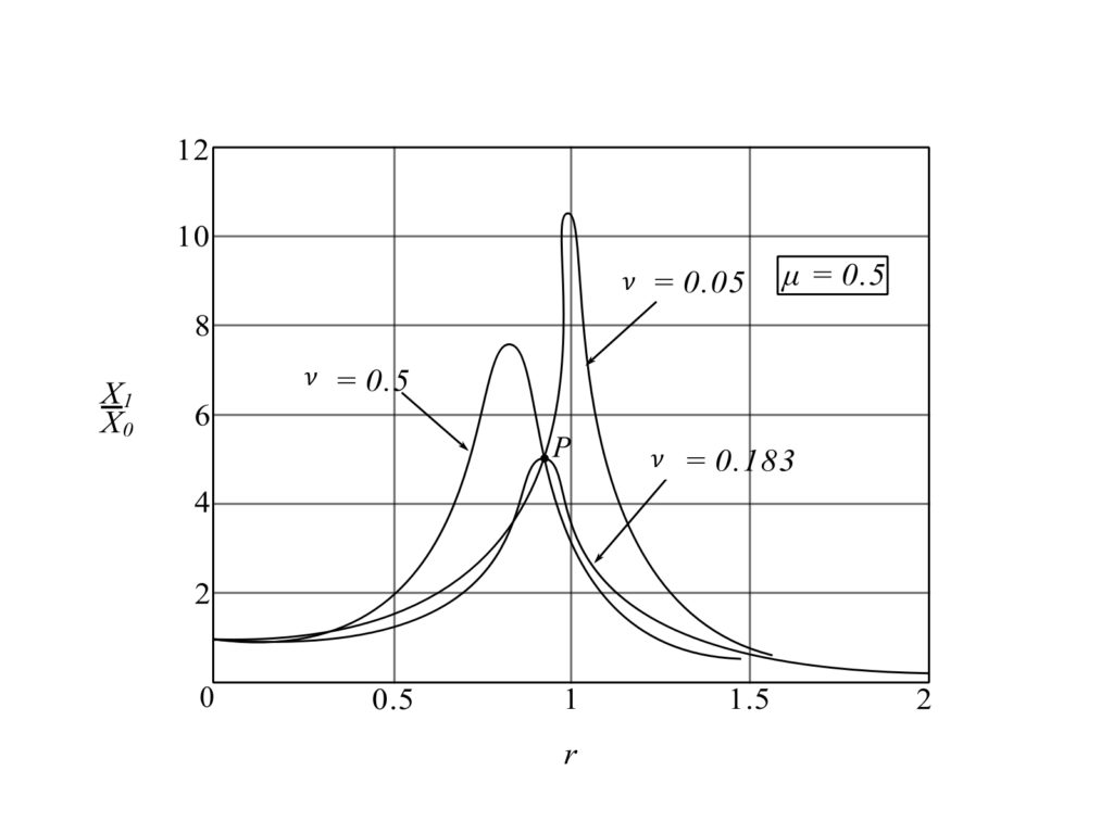
When  :
:
![\[\frac{X_1}{X_0} = \frac{\sqrt{\mu^2 + 4\nu^2}}{\sqrt{4\nu^2\mu^2}} \]](https://engcourses-uofa.ca/wp-content/ql-cache/quicklatex.com-a95f6f289d2e23842aee4eb5dda41ae7_l3.png "Rendered by QuickLaTeX.com")
When  :
:
![\[ \frac{X_1}{X_0} = \frac{\sqrt{ 0.25 + 4(0.365)^2}}{\sqrt{4(0.365)^2(\frac{1}{4})}} = 2.42\]](https://engcourses-uofa.ca/wp-content/ql-cache/quicklatex.com-cf20d71b1d945edc157340d92999d403_l3.png "Rendered by QuickLaTeX.com")
When  :
:
![\[\frac{X_1}{X_0} = \frac{\sqrt{0.25 + 4}}{\sqrt{4(1)(\frac{1}{4})}} = 2.06\]](https://engcourses-uofa.ca/wp-content/ql-cache/quicklatex.com-39f583f3f2167be53fa6e2ba224d8b8f_l3.png "Rendered by QuickLaTeX.com")
When  :
:
![\[\frac{X_1}{X_0} = \frac{\sqrt{0.25 + 0.04}}{\sqrt{4(0.01)(\frac{1}{4})}} = 5.39\]](https://engcourses-uofa.ca/wp-content/ql-cache/quicklatex.com-bdc6171be98eddd86e6ec5e5bc7da263_l3.png "Rendered by QuickLaTeX.com")
When  :
:
![\[\frac{X_1}{X_0} = \sqrt{\frac{0.25 + 4(0.1825)^2}{0.1825^2}} = 3.39 \]](https://engcourses-uofa.ca/wp-content/ql-cache/quicklatex.com-c74af7963355a9e22ed288f03a34c56b_l3.png "Rendered by QuickLaTeX.com")
Example
A second very practical application is the viciously damped vibration absorber.
Solution
From the general solution:
![\[ c_1 = 0,\ c_2 = C \]](https://engcourses-uofa.ca/wp-content/ql-cache/quicklatex.com-3ce21802b40f29205221b2052d188d91_l3.png "Rendered by QuickLaTeX.com")
Therefore:
![\[V_{11} = m_1s^2 + cs + k_1 + k_2 \]](https://engcourses-uofa.ca/wp-content/ql-cache/quicklatex.com-0b0459c80e587733f1a8932b30676ca5_l3.png "Rendered by QuickLaTeX.com")
![\[V_{12} = - (cs + k_2) = V_{21}\]](https://engcourses-uofa.ca/wp-content/ql-cache/quicklatex.com-c371fbab0d4f62f310b161e9ebc9e780_l3.png "Rendered by QuickLaTeX.com")
![\[V_{22} = m_2s^2 + cs + k_2 \]](https://engcourses-uofa.ca/wp-content/ql-cache/quicklatex.com-db8b6d5bef15170f387b157b18adb871_l3.png "Rendered by QuickLaTeX.com")
![\[ \zeta_1 = Y_{11}f_1 ,\ \zeta_2 = Y_{21}f_1 \]](https://engcourses-uofa.ca/wp-content/ql-cache/quicklatex.com-eeb6c11b43c3c501e52599dcd3bf813e_l3.png "Rendered by QuickLaTeX.com")
![\[Y_{11} = \frac{V_{22}}{\Delta},\ Y_{21} = -\frac{V_{12}}{\Delta} \]](https://engcourses-uofa.ca/wp-content/ql-cache/quicklatex.com-81bee900a0c5d195bbab8c04725b2d09_l3.png "Rendered by QuickLaTeX.com")
![\[\Delta = \big[ - m_1\omega^2 + ic\omega +k_1 + k_2\big] \big[-m_2\omega^2 + ic\omega + k_2 \big] - \big[k_2 + ic\omega\big]^2\]](https://engcourses-uofa.ca/wp-content/ql-cache/quicklatex.com-fbd870df7a675d412ab82689a24b0a35_l3.png "Rendered by QuickLaTeX.com")
![\[\implies \Delta = \big[(-m_1\omega^2 + k_1)(-m_2\omega^2 + k_2) - m_2\omega^2 k_2\big] + ic\omega[-m_1\omega^2 + k_1 - m_2\omega^2]\]](https://engcourses-uofa.ca/wp-content/ql-cache/quicklatex.com-56ff5ba5747745a8df898a34ac440aba_l3.png "Rendered by QuickLaTeX.com")
![\[ \zeta_1 = Y_{11}F_0e^{i\omega t} = \frac{(-m_2\omega^2 + ic\omega + k_2)}{\Delta}F_0e^{i\omega t}\]](https://engcourses-uofa.ca/wp-content/ql-cache/quicklatex.com-03f19187b91402b7b4d8c8d600069d66_l3.png "Rendered by QuickLaTeX.com")
If we set  :
:
![\[ (\frac{X_1}{F_0})^2 = \frac{(k_2 - m_2\omega^2)^2 +\omega^2c^2}{\Delta \bar{\Delta}}\]](https://engcourses-uofa.ca/wp-content/ql-cache/quicklatex.com-1103e0dccd6c12b06baa666ad2091d48_l3.png "Rendered by QuickLaTeX.com")
![\[\begin{split}\zeta_2 &= Y_{21}f_1 \\&= \frac{k_2 + ic\omega}{\Delta \bar{\Delta}} \\&= X_2e^{i\theta_2} \end{split}\]](https://engcourses-uofa.ca/wp-content/ql-cache/quicklatex.com-5cff66251d2a6612779286818f2b5744_l3.png "Rendered by QuickLaTeX.com")
![\[(\frac{X_2}{F_0})^2 = \frac{k_2^2+c^2\omega^2}{\Delta \bar{\Delta}}\]](https://engcourses-uofa.ca/wp-content/ql-cache/quicklatex.com-bc02a446ad8415f148a30f3d9603fe1d_l3.png "Rendered by QuickLaTeX.com")
In order to apply this to various situations, it is useful to non-dimensionalize these relationships similar to that of the undamped vibration absorber.
Set:
![\[X_0 = \frac{F_0}{k_1},\ \nu = \frac{c}{2m_2p_{11}} \]](https://engcourses-uofa.ca/wp-content/ql-cache/quicklatex.com-d199baf27af63e79c5eefe734976d0ee_l3.png "Rendered by QuickLaTeX.com")
![\[p_{11} = \sqrt{\frac{k_1}{m_1}},\ p_{22} = \sqrt{\frac{k_2}{m_2}} \]](https://engcourses-uofa.ca/wp-content/ql-cache/quicklatex.com-1d0f1bcff12c3daaa24a5c53d8e81899_l3.png "Rendered by QuickLaTeX.com")
NOTE:
![\[(\omega c)^2 = \bigg( \frac{\omega}{p_{11}^2}c\frac{k_1}{m_1}\bigg)^2\]](https://engcourses-uofa.ca/wp-content/ql-cache/quicklatex.com-f06441768152b9dfa52f4907b6da5719_l3.png "Rendered by QuickLaTeX.com")
![\[ r = \frac{\omega}{p_{11}},\ \mu = \frac{m_2}{m_1} \]](https://engcourses-uofa.ca/wp-content/ql-cache/quicklatex.com-fb70f3c9fbc6ab4c45c84e5fbaa2d523_l3.png "Rendered by QuickLaTeX.com")
Therefore:
![\[ (\omega c)^2 = \bigg[ \frac{\omega}{p_{11}}2\frac{c}{2m_2p_{11}}\mu^2k_1\frac{m_1}{m_2}\bigg]^2 = k_1^2\mu^2[2\nu r]^2 \]](https://engcourses-uofa.ca/wp-content/ql-cache/quicklatex.com-d7570a7b2beb2738fc7a6b777def54c9_l3.png "Rendered by QuickLaTeX.com")
![\[ \begin{split}(k_2 - m_2\omega^2)^2 &= k_1^2\bigg[\frac{k_2}{k_1} - \frac{m_2\omega^2}{k_1} \bigg] ^2 \\&= \bigg[\frac{m_1}{m_2}\frac{k_2}{k_1}\frac{m_2}{m_1} - \frac{m_2}{m_1}\omega^2 \frac{m_1}{k_1}\bigg]^2k_1^2 \\&= \mu^2k_1^2[r^2 - g^2]^2 \end{split}\]](https://engcourses-uofa.ca/wp-content/ql-cache/quicklatex.com-b71b9306baf1b150f09f78f6d6da0eb5_l3.png "Rendered by QuickLaTeX.com")
![\[ g = \frac{p_{22}}{p_{11}} \]](https://engcourses-uofa.ca/wp-content/ql-cache/quicklatex.com-e154d0357d5f72890387c01619f70525_l3.png "Rendered by QuickLaTeX.com")
![\[ \begin{split}\Delta \bar{\Delta} &= \big[(-m_1\omega^2 + k_1)(-m_2\omega^2 + k_2) - m_2\omega^2 k_2 \big] ^2 + c^2\omega^2[-m_1\omega^2 + k_1 - m_2 \omega^2 \big] ^2 \\&= (2\nu r)^2[r^2 - 1 + \mu r^2]^2 + \big[\mu g^2r^2 - (r^2-1)(r^2-g^2)\big]^2\end{split}\]](https://engcourses-uofa.ca/wp-content/ql-cache/quicklatex.com-6710b492fa252200ed4e47802591c006_l3.png "Rendered by QuickLaTeX.com")
![\[ \frac{X_1}{X_0} = \sqrt{\frac{(2\nu r)^2 + ( r^2 - g^2)^2}{(2\nu r)^2(r^2 - 1 + \mu r^2)^2 + \big[\mu g^2r^2 - (r^2-1)(r^2-g^2)\big]^2}} \]](https://engcourses-uofa.ca/wp-content/ql-cache/quicklatex.com-b8af8d9a307a2690f39612fa9d238be3_l3.png "Rendered by QuickLaTeX.com")
![\[ \mu = \frac{m_2}{m_1} \quad \text{(mass ratio)}\]](https://engcourses-uofa.ca/wp-content/ql-cache/quicklatex.com-a6632175e28ef6b73fe68cfd824cf613_l3.png "Rendered by QuickLaTeX.com")
![\[ \nu = \frac{c}{2m_2p_{11}} \quad \text{(damping ratio)} \]](https://engcourses-uofa.ca/wp-content/ql-cache/quicklatex.com-6118020843121bf16225ebb5f76ab4fb_l3.png "Rendered by QuickLaTeX.com")
![\[g = \frac{p_{22}}{p_{11}} \quad \text{(frequency ratio of subsystems)}\]](https://engcourses-uofa.ca/wp-content/ql-cache/quicklatex.com-dbe86cb8e2c6eeb26b27aa2d74fa2d5b_l3.png "Rendered by QuickLaTeX.com")
![\[r = \frac{\omega}{p_{11}} \]](https://engcourses-uofa.ca/wp-content/ql-cache/quicklatex.com-6480df489f785efb2c10692b36967a97_l3.png "Rendered by QuickLaTeX.com")
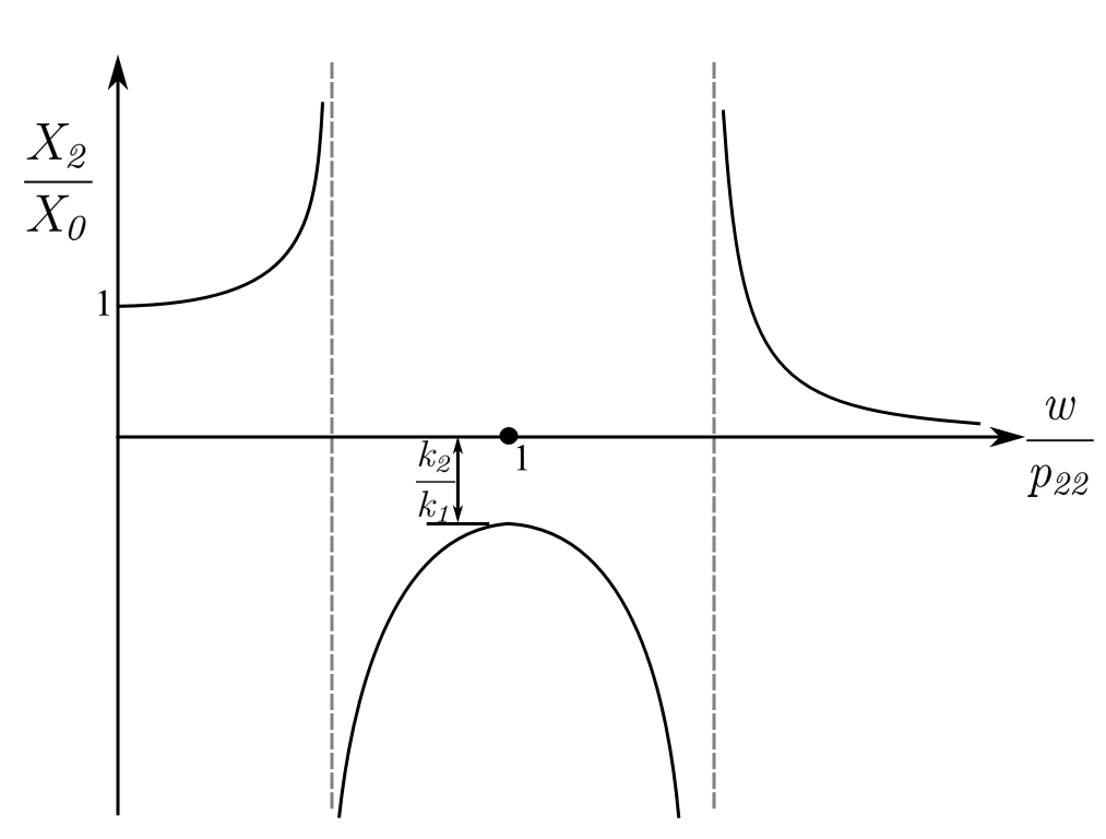
![\[ \frac{X_2}{X_0} = \frac{\mu r\sqrt{1+4\nu^2}}{\sqrt{(2\nu r)^2(r^2 - 1 +\mu r^2)^2 + \big[\mu g^2r^2 - ( r^2 - 1)(r^2 - g^2)\big]^2}}\]](https://engcourses-uofa.ca/wp-content/ql-cache/quicklatex.com-dda52f02de41658a31e1a2327086df97_l3.png "Rendered by QuickLaTeX.com")
CHECK
- If
 :
:![\[\frac{X_1}{X_0} = \frac{r^2 - g^2}{\mu g^2r^2 - (r^2 - 1)(r^2 - g^2)} \]](https://engcourses-uofa.ca/wp-content/ql-cache/quicklatex.com-40d79fc1a7f220c16ef0f45c35167009_l3.png "Rendered by QuickLaTeX.com")
- If
 , then
Note that only when
If :
:![\[ \begin{split}\frac{X_1}{X_0} &= \frac{1}{r^2 - 1 + \mu r^2} \\&= \frac{1}{(1+\mu)r^2-1} \\&= \frac{1}{\frac{m_1 + m_2}{k_1}\omega^2 -1} \end{split}\]](https://engcourses-uofa.ca/wp-content/ql-cache/quicklatex.com-7f2358da89a26903bfad3a658f318a24_l3.png "Rendered by QuickLaTeX.com")
As a result somewhere between  and ,
and ,  will give an optimal result.
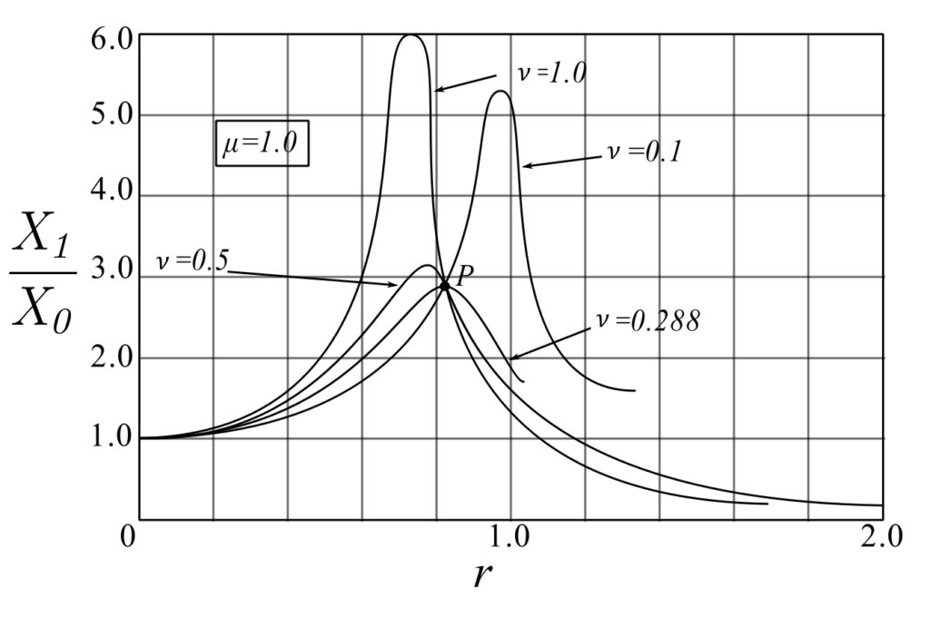
Note that all the curves intersect at  and
and  . That is these points are independent of the damping. If we calculate their location, our problem is essentially solved as we must find the curve that passes through them with a horizontal tangent. Also by changing the “tuning”
  the two points can be shifted up and down the
  curve. We can do this until the two points have the same height and the horizontal tangent through one of them.
To find the two points where the amplitude is independent of the damping  and this is independent when
  :
:
![\[\bigg(\frac{1}{r^2 - 1 + \mu^2r^2}\bigg)^2 = \bigg[ \frac{(r^2-g^2)^2}{\mu g^2r^2 - (r^2-1)(r^2 - g^2)}\bigg]^2 \]](https://engcourses-uofa.ca/wp-content/ql-cache/quicklatex.com-c7e2798665a26a59fde3fc301c390b76_l3.png "Rendered by QuickLaTeX.com")
This leads to:
![\[ \mu g^2r^2 - (r^2-1)(r^2-g^2) = \pm(r^2-g^2)(r^2 - 1 + \mu r^2) \]](https://engcourses-uofa.ca/wp-content/ql-cache/quicklatex.com-3d3ad5d3db3d986a684371f6ea5da946_l3.png "Rendered by QuickLaTeX.com")
The negative gives  while the positive gives
  .
.
The two answers for the forcing frequency ratio are functions of  and but not of the damping .
We now wish to adjust so that & are equal. Since their magnitude is independent of the damping, choose  then the magnitude:
![\[\frac{X_1}{X_0} = \frac{1}{\mu r^2 + r^2 - 1} \]](https://engcourses-uofa.ca/wp-content/ql-cache/quicklatex.com-c3b7b2367c44f08ea36a3d0de1b3a97e_l3.png "Rendered by QuickLaTeX.com")
For  and
and  (the two roots), we want the same magnitude:
![\[ \frac{1}{\mu r_1^2 + r_1^2 - 1} = -\frac{1}{\mu r_2^2 + r_2^2 - 1}\]](https://engcourses-uofa.ca/wp-content/ql-cache/quicklatex.com-cfa2e966dce0862ea2d8568db0fa6c10_l3.png "Rendered by QuickLaTeX.com")
Therefore:
![\[1 - (\mu + 1) r_2^2 = -1 + (\mu + 1) r_1^2\]](https://engcourses-uofa.ca/wp-content/ql-cache/quicklatex.com-d28e1a5975ea8959a25094ef564ff96b_l3.png "Rendered by QuickLaTeX.com")
![\[ \frac{2}{1+\mu} = r_1^2 + r_2^2 \]](https://engcourses-uofa.ca/wp-content/ql-cache/quicklatex.com-cc372f89d2ed677f3d199937549d3682_l3.png "Rendered by QuickLaTeX.com")
Now it is not necessary to solve for and if we remember the sum of the roots in a quadratic in the negative coefficient of the middle term.
Therefore:
![\[ \frac{2}{1+\mu} = \frac{2(1+g^2+\mu g^2)}{2+\mu} \]](https://engcourses-uofa.ca/wp-content/ql-cache/quicklatex.com-ea264d1ade3d2464844c33025aa598d3_l3.png "Rendered by QuickLaTeX.com")
![\[ \frac{2+\mu}{1+\mu} = 1+ g^2(1+\mu) \]](https://engcourses-uofa.ca/wp-content/ql-cache/quicklatex.com-919d3e7c365b844a52000cd8f3ac3f24_l3.png "Rendered by QuickLaTeX.com")
![\[\begin{split} \implies g^2(1+\mu) &= \frac{2+\mu - 1 - \omega}{1+ \mu} \\&= \frac{1}{1+\mu} \end{split}\]](https://engcourses-uofa.ca/wp-content/ql-cache/quicklatex.com-f17f55c2efdd5ae4b19f6548b578065c_l3.png "Rendered by QuickLaTeX.com")
Therefore:
![\[g = \frac{1}{1+\mu} \]](https://engcourses-uofa.ca/wp-content/ql-cache/quicklatex.com-fc238912ecd93c6adc58586021867eff_l3.png "Rendered by QuickLaTeX.com")
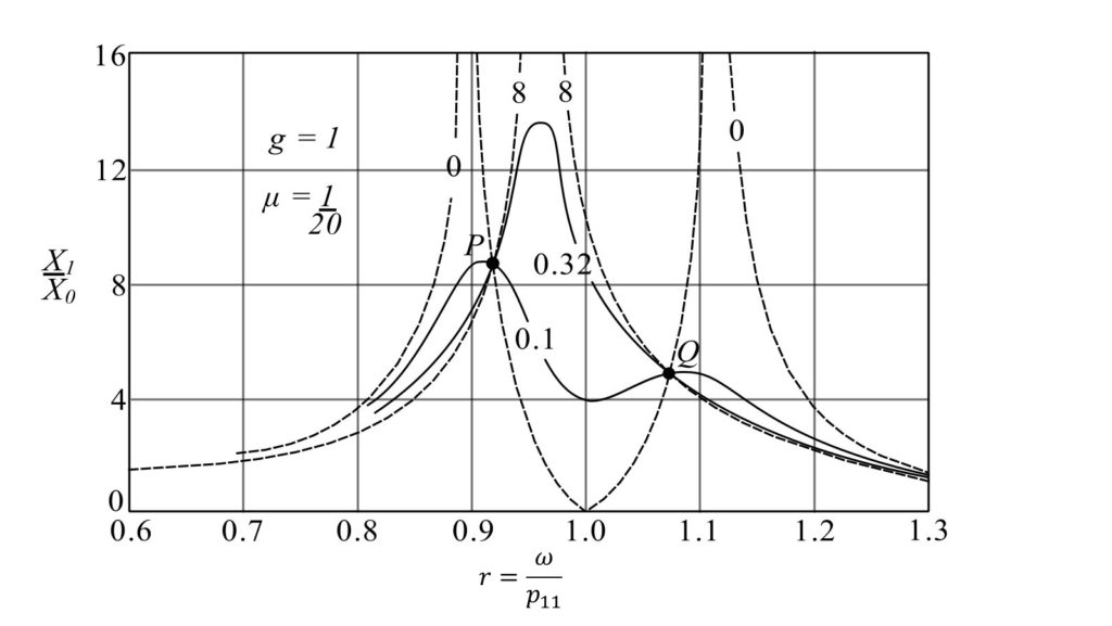
Amplitudes of the main mass for various values of absorber damping. The absorber is twenty times as small as the main machine and is tuned to the same frequency. All curves pass through the fixed points and .
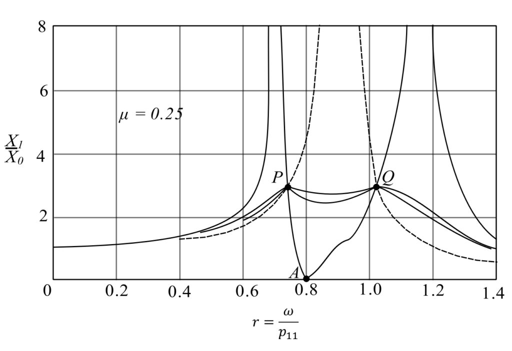
Resonance curves for the motion of the main mass fitted with the most favorably tuned vibration-absorber system of one-forth of the size of the main machine.
(a)
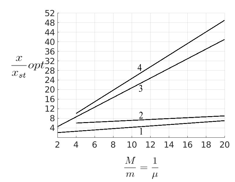
(b)
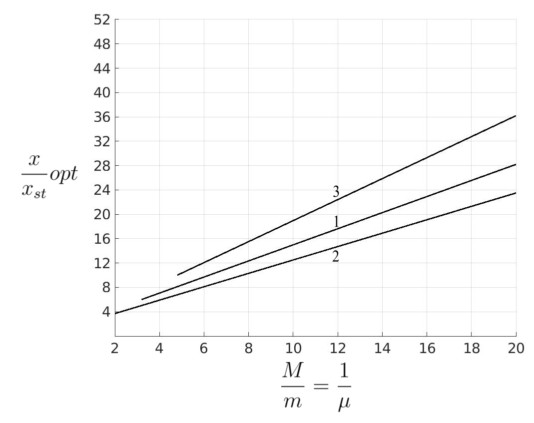
(c)
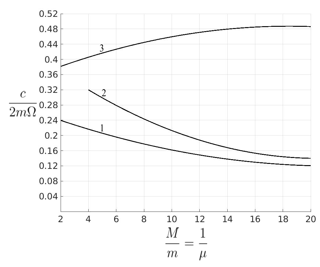
(a) Peak amplitudes of the main mass as a function of the ratio  for various absorbers attached to the main mass. (b) Peak relative amplitudes between the masses
  and
and  for various absorbers. (c) Damping constants required for the most favorable operation of the absorber,
  , for obtaining the results of (a) and (b).
Curve 1 for the most favorably tuned and damped absorber; curve 2 for the most favorably damped absorber tuned to the frequency of the main system; curve 3 of the most favorably damped viscous Lanchester damper; curve 4 for the most favorably damped Coulomb Lanchester damper.
![\[ \bigg(\frac{X_1}{X_0}\bigg)_\text{MAX} = \frac{1}{1-r^2(1+\mu)}\]](https://engcourses-uofa.ca/wp-content/ql-cache/quicklatex.com-bea09eddc963019253b32d04e7efc4ff_l3.png "Rendered by QuickLaTeX.com")
and using one of the roots:
![\[ \bigg(\frac{X_1}{X_0}\bigg)_\text{MAX} = \sqrt{1+ \frac{2}{\mu}} \]](https://engcourses-uofa.ca/wp-content/ql-cache/quicklatex.com-a99b95a6c5e3c17d754939e712f20c17_l3.png "Rendered by QuickLaTeX.com")
while the optimum damping is given by:
![\[ \nu = \sqrt{\frac{3\mu}{8(1+\mu)^3}} \]](https://engcourses-uofa.ca/wp-content/ql-cache/quicklatex.com-c958127705b0c83d08ba8be337f6dd33_l3.png "Rendered by QuickLaTeX.com")