
Review of single and multi-degree of freedom (mdof) systems: Transient Vibrations
For dynamical systems excited by non-periodic forces, displacements, accelerations, etc., the response over the initial few periods of the system is termed transient response. This is important for many diverse situations including packaging of equipment, protecting people from automobile impacts, and loading of structures due to blasts and earthquakes. The modeling of these situations is often difficult and may require specific detail of the excitation as the response can vary dramatically depending on the detail of the input.
For a SDOF system the solution requires the general solution of  and becomes difficult for complicated
Example
Consider first the undamped case for a step input:
Solution
![\[ m\ddot{x} +kx = F_0, t>0\]](https://engcourses-uofa.ca/wp-content/ql-cache/quicklatex.com-26e5075479581911c15c3d17ddc66dd8_l3.png "Rendered by QuickLaTeX.com")
![\[ \implies x_H = A\sin{pt} + B\cos{pt} \]](https://engcourses-uofa.ca/wp-content/ql-cache/quicklatex.com-ba56b8b16f7353825a344d5ce49a1d59_l3.png "Rendered by QuickLaTeX.com")
Assume 
![\[ \implies kC = F_0 \]](https://engcourses-uofa.ca/wp-content/ql-cache/quicklatex.com-183516c0393306702a17893da985bb5c_l3.png "Rendered by QuickLaTeX.com")
![\[C = \frac{F_0}{k} \]](https://engcourses-uofa.ca/wp-content/ql-cache/quicklatex.com-5de55aece7320f39ec2b8305ec1b3a89_l3.png "Rendered by QuickLaTeX.com")
and the total solution:
![\[\begin{split} x(t) &= x_H +x_p \\&= \frac{F_0}{k} + A\sin{pt} + B \cos{pt} \end{split} \]](https://engcourses-uofa.ca/wp-content/ql-cache/quicklatex.com-a5160ccacfe3857f0b89374f0035d17a_l3.png "Rendered by QuickLaTeX.com")
If  , then:
![\[ B = -\frac{F_0}{k} \]](https://engcourses-uofa.ca/wp-content/ql-cache/quicklatex.com-b90cd31900076f9038d3f2b0cc59dfad_l3.png "Rendered by QuickLaTeX.com")
![\[A = 0 \]](https://engcourses-uofa.ca/wp-content/ql-cache/quicklatex.com-af872ffa59db9a38073ae57ffe7b5842_l3.png "Rendered by QuickLaTeX.com")
![\[x(t) = \frac{F_0}{k}(1-\cos{pt}) \]](https://engcourses-uofa.ca/wp-content/ql-cache/quicklatex.com-a3be44792be7561111810c051130b80f_l3.png "Rendered by QuickLaTeX.com")
While this case is straightforward, the solution is more difficult with damping or for different forcing functions.
The response can be determined in a general form by considering as being made up from a series of short impulses. A general short impulse at some time  is shown. Consider what happens(response) if only this impulse is applied to the system:
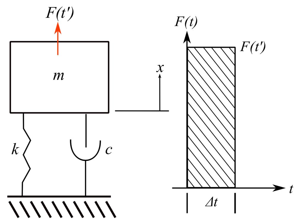
If  is vanishingly small the impulse can be considered as changing the velocity of
  using impulses/momentum relations so that from initial
  (just before) to final
 condition:
![\[(m\dot{x})_i + F(t')\Delta t = (m\dot{x})_F \]](https://engcourses-uofa.ca/wp-content/ql-cache/quicklatex.com-7523d3158f1469da69c26c8027dd5f2c_l3.png "Rendered by QuickLaTeX.com")
Therefore:
![\[ \dot{x}_F - \dot{x}_i = \frac{F_0(t')}{m}\Delta t \]](https://engcourses-uofa.ca/wp-content/ql-cache/quicklatex.com-8556212533569a11a8a5f7955456f579_l3.png "Rendered by QuickLaTeX.com")
This impulses will result in a free vibration with initial conditions:
![\[ x(0) = 0 \]](https://engcourses-uofa.ca/wp-content/ql-cache/quicklatex.com-788ae18e8265931b8433533a97e9ce4e_l3.png "Rendered by QuickLaTeX.com")
![\[\dot{x}(0) = \frac{F(t')}{m} \Delta t\]](https://engcourses-uofa.ca/wp-content/ql-cache/quicklatex.com-356bed42020a204a9c38abbd151ca333_l3.png "Rendered by QuickLaTeX.com")
If this is the only impulse then the response is:
![\[ x(t) = e\strut^{-\zeta pt}\big[A\cos{\sqrt{1-\zeta^2}pt} + B\sin{\sqrt{1-\zeta^2}pt}\big] \]](https://engcourses-uofa.ca/wp-content/ql-cache/quicklatex.com-c8eaf18acd27174a3b24499443fbbb8e_l3.png "Rendered by QuickLaTeX.com")
with 
![\[ \implies A=0 \]](https://engcourses-uofa.ca/wp-content/ql-cache/quicklatex.com-5bdaff5daf8b9387c0d4d5372edd673a_l3.png "Rendered by QuickLaTeX.com")
![\[ \begin{split}\dot{x}(0) &= B\sqrt{1-\zeta^2}p \\&= \frac{F(t')}{m}\Delta t \end{split}\]](https://engcourses-uofa.ca/wp-content/ql-cache/quicklatex.com-2d639496b4402aab9624a378d7ae1dfb_l3.png "Rendered by QuickLaTeX.com")
![\[ \implies B = \frac{F(t')\Delta t}{mp\sqrt{1=\zeta^2}} \]](https://engcourses-uofa.ca/wp-content/ql-cache/quicklatex.com-88e828a378e52615c4e66b5a03e2a07c_l3.png "Rendered by QuickLaTeX.com")
Therefore:
![\[x(t) = \frac{F(t') \Delta t}{mp\sqrt{1-\zeta^2}}e^{-\zeta pt}\sin{\big(\sqrt{1-\zeta^2}pt\big)} \]](https://engcourses-uofa.ca/wp-content/ql-cache/quicklatex.com-88d7b21a54a5ea703a94d9f7a1dc16ce_l3.png "Rendered by QuickLaTeX.com")
Where  is the time since the impulse.
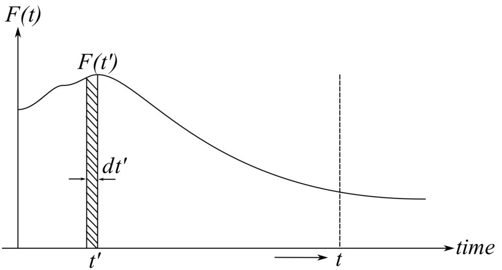
Therefore the response at due to the impulse at is  :
:
![\[x'(t) = \frac{F(t')\Delta t'e^{-\zeta p(t-t')}}{mp\sqrt{1-\zeta^2}}\sin{\big[\sqrt{1-\zeta^2}p(t-t')\big]}\]](https://engcourses-uofa.ca/wp-content/ql-cache/quicklatex.com-1195b07563d8c35762f742f4f03fb7f3_l3.png "Rendered by QuickLaTeX.com")
The response due to all the impulses from  to
to  is the superposition of all the impulses’ response.
Therefore:
![\[x(t) = \frac{1}{mp\sqrt{1-\zeta^2}} \int _0^\tau F(t')e^{-\zeta p(t-t')}\sin{\sqrt{1-\zeta^2}p(t-t')}\,dt'\]](https://engcourses-uofa.ca/wp-content/ql-cache/quicklatex.com-b20b51656a2d89b12a97cf5051a7092c_l3.png "Rendered by QuickLaTeX.com")
Assuming  i.e. the mass was stationary prior to being applied.
For the step input 
![\[x(t) = \frac{F_0}{k}\biggr[1-\frac{e^{-\zeta pt}}{\sqrt{1-\zeta^2}}\cos{\big(\sqrt{1-\zeta^2}pt - \Psi\big)}\biggr]\]](https://engcourses-uofa.ca/wp-content/ql-cache/quicklatex.com-93a6b7033b6a0d25a6bf3691b5200de6_l3.png "Rendered by QuickLaTeX.com")
![\[ \tan{\psi} = \frac{\zeta}{\sqrt{1=\zeta^2}}\]](https://engcourses-uofa.ca/wp-content/ql-cache/quicklatex.com-f08f82a346214ecc0d8a873859512bb8_l3.png "Rendered by QuickLaTeX.com")
If the initial conditions are  , then:
![\[\begin{split}x(t) &= e\strut^{-\zeta pt}\biggr[x_0\cos{\sqrt{1-\zeta^2}}pt+\frac{v_0 + \zeta px_0}{\sqrt{1-\zeta^2}p}\sin{\sqrt{1-\zeta^2}pt}\biggr] \\&+\frac{1}{mp\sqrt{1-\zeta^2}} \int _0^\tau F(t')e^{\zeta p(t-t')}\sin{\sqrt{1-\zeta^2}p(t-t')}\,dt'\end{split} \]](https://engcourses-uofa.ca/wp-content/ql-cache/quicklatex.com-7f98fb0add8397760cdf92e15d4eec74_l3.png "Rendered by QuickLaTeX.com")
Example
For a package being dropped or for an airplane landing, a SDOF model can be utilized.
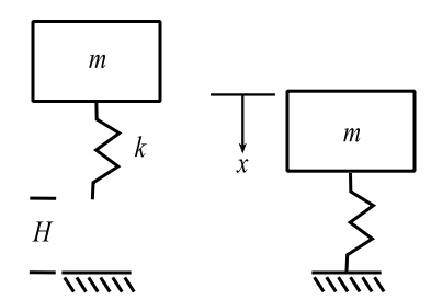
For the undamped case, as it strikes,  and
and  , and the forcing function is
  (constant). NOTE:
  is not measured from the static equilibrium configuration. Using the general result:
![\[ \begin{split} x(t) &= \frac{\sqrt{2gH}}{p}\sin pt +\frac{1}{mp} \int_{0}^{t} mg\sin (t-t') dt' \\&= \frac{\sqrt{2gH}}{p}\sin pt + \frac{g}{p} \Big[\frac{\cos p(t-t')}{p}\Big]_{o}^{t} \\&= \frac{\sqrt{2gH}}{p}\sin pt + \frac{g}{p^2}\Big[1 - \cos pt \Big] \end{split} \]](https://engcourses-uofa.ca/wp-content/ql-cache/quicklatex.com-ba2457ab77d3ffbd9a9a4091584a6065_l3.png "Rendered by QuickLaTeX.com")
![\[x(t) = \sqrt{\frac{2gH}{p^2} + \Big(\frac{g}{p^2}\Big)^2} \sin(pt + \phi) + \frac{g}{p^2}\]](https://engcourses-uofa.ca/wp-content/ql-cache/quicklatex.com-bc423e314452d16e94f70981715facef_l3.png "Rendered by QuickLaTeX.com")
![\[\ddot{x}(t) = -p^2\sqrt{\frac{2gH}{p^2} + \Big(\frac{g}{p^2}\Big)^2} \sin(pt + \phi) \]](https://engcourses-uofa.ca/wp-content/ql-cache/quicklatex.com-f4e85ecf7dc11adb6e5adc902e9fcc93_l3.png "Rendered by QuickLaTeX.com")
Therefore, the maximum acceleration is:
![\[ \frac{\ddot{x}_\text{MAX}}{g} = -\frac{1}{\delta_\text{ST}}\sqrt{2H\delta_\text{ST} + \delta_\text{ST}^2} \]](https://engcourses-uofa.ca/wp-content/ql-cache/quicklatex.com-7358954915e76b877dade6b42bb0cd0b_l3.png "Rendered by QuickLaTeX.com")
![\[ \frac{\ddot{x}_\text{MAX}}{g} = -\sqrt{\frac{2H}{\delta_\text{ST}} + 1} \]](https://engcourses-uofa.ca/wp-content/ql-cache/quicklatex.com-587c3c4f2b84b8d77bee1c9410605325_l3.png "Rendered by QuickLaTeX.com")
With:
![\[\begin{split} \delta_\text{ST} &= \frac{mg}{k} \\ &= \frac{p}{g^2} \end{split}\]](https://engcourses-uofa.ca/wp-content/ql-cache/quicklatex.com-2607cb4f31fe536cb3b364400708c7ec_l3.png "Rendered by QuickLaTeX.com")
In forensic studies of automobile collisions, the concern is the acceleration of a passenger’s head and the potential for internal damage. Assume the body/skull is modelled as a SDOF system.
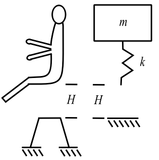
Biomechanical studies gives the spinal stiffness  . Assume the person weighs 160 lbs and falls 6 inches because of being unrestrained. Thus:
![\[\begin{split} \delta_\text{ST} &= \frac{160}{458} \\&= 0.35 \ \text{inches} \end{split} \]](https://engcourses-uofa.ca/wp-content/ql-cache/quicklatex.com-b01e42aa49eddcdabc367b91c2b45ea5_l3.png "Rendered by QuickLaTeX.com")
Therefore:
![\[ \begin{split} \frac{\ddot{x}_\text{MAX}}{g} &= -\sqrt{\frac{12}{0.35} + 1} \\&= -5.94 \end{split} \]](https://engcourses-uofa.ca/wp-content/ql-cache/quicklatex.com-4237cd444ccae1b652dbe22e98277fe2_l3.png "Rendered by QuickLaTeX.com")
If we add a seat cushion to the seat (cushion stiffness is  ). What is the change in maximum acceleration?
The effective stiffness is now:
![\[\frac{1}{k_\text{eff}} = \frac{1}{458} + \frac{1}{51}\]](https://engcourses-uofa.ca/wp-content/ql-cache/quicklatex.com-d01deaf8d7f01d727fa540e8867c0e0e_l3.png "Rendered by QuickLaTeX.com")
![\[\begin{split} k_\text{eff} &= \frac{(51)(458)}{458 + 51} \\& = \ 45.9 \text{ lbs/in} \end{split}\]](https://engcourses-uofa.ca/wp-content/ql-cache/quicklatex.com-eba28e2de0545a9aea1c39a21c42da13_l3.png "Rendered by QuickLaTeX.com")
Thus:
![\[\begin{split} \delta_\text{ST} &= \frac{160}{45.9} \\&= 3.49 \ \text{in} \end{split}\]](https://engcourses-uofa.ca/wp-content/ql-cache/quicklatex.com-d6bd723edea0439f5058931cf8e9b760_l3.png "Rendered by QuickLaTeX.com")
Therefore:
![\[ \begin{split} \frac{\ddot{x}_\text{MAX}}{g} &= -\sqrt{\frac{12}{3.49} + 1} \\&= -2.1 \end{split} \]](https://engcourses-uofa.ca/wp-content/ql-cache/quicklatex.com-1627ed10a2f2d9700b8846801ca5f637_l3.png "Rendered by QuickLaTeX.com")
The cushion reduces the acceleration drastically.
For many situations, the support of the system is subjected to the motion specified by its displacement, velocity, or acceleration.
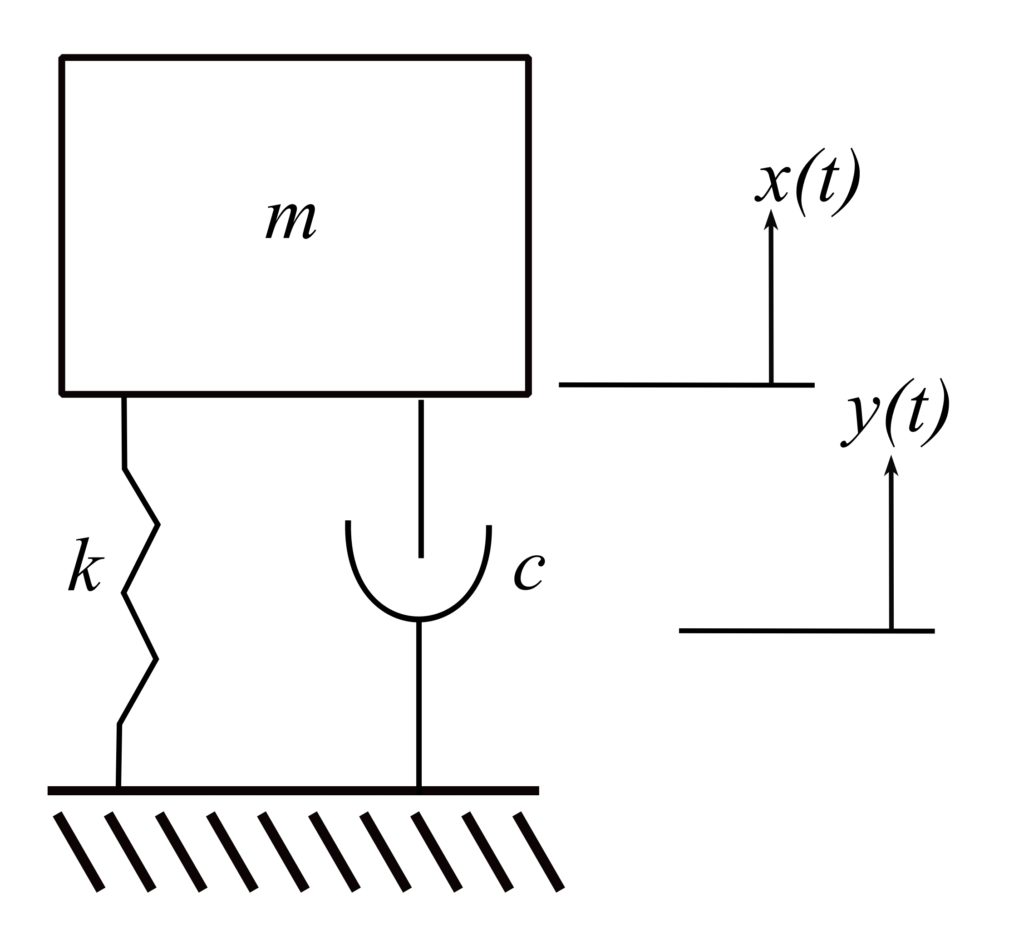
Therefore, for base acceleration:
![\[ m\ddot{x}+ k(x-y) + c(\dot{x} - \dot{y}) = 0 \]](https://engcourses-uofa.ca/wp-content/ql-cache/quicklatex.com-41999cdb2502233da7f901b6f9f03efe_l3.png "Rendered by QuickLaTeX.com")
![\[m(\ddot{x} - \ddot{y}) + k(x-y) + c(\dot{x} - \dot{y}) = -m\ddot{y}\]](https://engcourses-uofa.ca/wp-content/ql-cache/quicklatex.com-991ab6517c6b9acf30e5c9a8c7466908_l3.png "Rendered by QuickLaTeX.com")
Using the relative displacement  :
:
![\[m\ddot{z} + c\dot{z} + kz = -m\ddot{y} \]](https://engcourses-uofa.ca/wp-content/ql-cache/quicklatex.com-8b691943a08ab180b61ad20e15f0bd14_l3.png "Rendered by QuickLaTeX.com")
The convolution integral for this case is:
![\[ z(t) = -\frac{1}{\sqrt{1-\zeta^2}p}\int_0^t \ddot{y}(t') e^{-\zeta(t-t')}\sin\sqrt{1-\zeta^2}p(t-t') dt' \]](https://engcourses-uofa.ca/wp-content/ql-cache/quicklatex.com-cc3f0b8c4b50aa19ca6b52f7ef33b8c8_l3.png "Rendered by QuickLaTeX.com")
The same approach can be used for a base excitation with velocity.
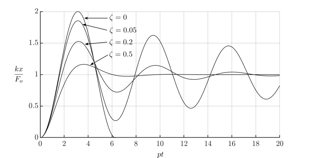
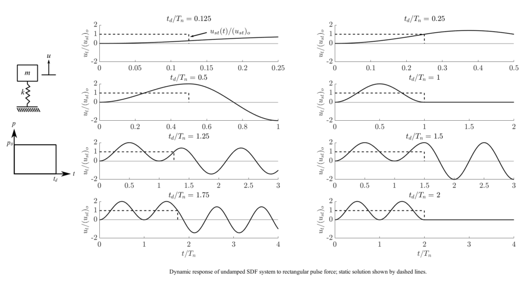
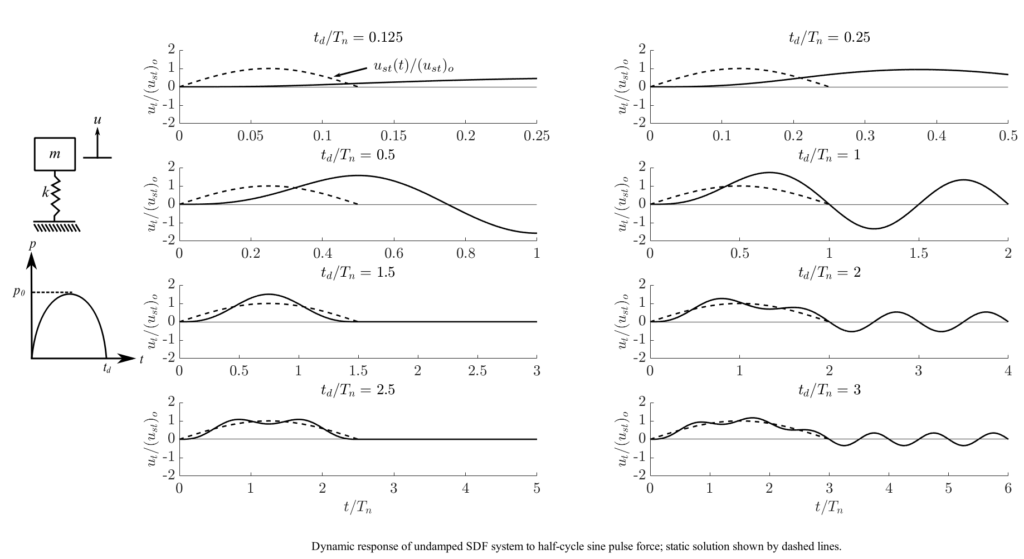
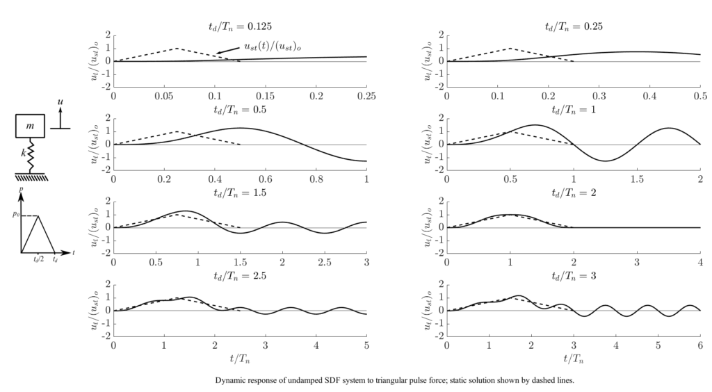
Examples of Dynamic Responses of Undamped SDF Systems to Different Pulse Forces
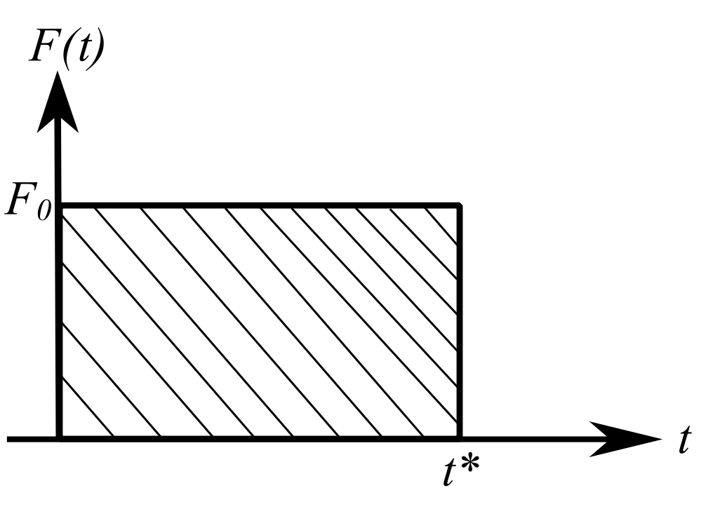
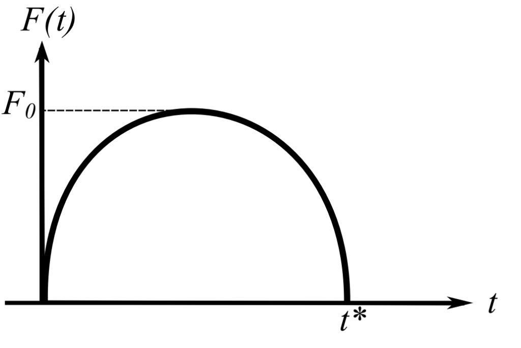
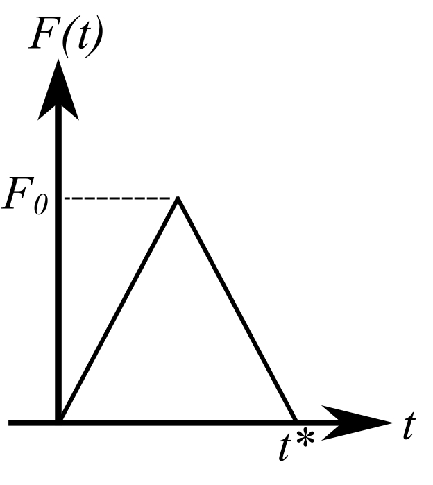
Note that the static solution is shown in the dashed lines.
Rectangular Pulse Force
Half Cycle Sine Pulse Force
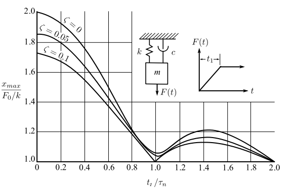
Triangular Pulse Force
Shock Response Spectrum
Previously we developed a technique to find the response of a damped spring mass system to an arbitrary excitation. When the duration of the pulse is small compared to the natural period ( ), the excitation is called a shock. It has been found that the concept of the shock response spectrum is useful for these situations.
The Shock Response Spectrum (SRS) is a plot of the maximum peak response of a SDOF oscillator as a function of the natural period of the oscillator. The maximum of the peaks (called maxima) represents only a single point on the time response curve.
To illustrate the SRS concept consider a SDOF undamped system with no initial motion  . The SRS is
![\[ x(t)\bigg|_\text{MAX}=\bigg|\frac{1}{mP}\int_0^t F(t')\sin p(t-t')dt'\bigg|_\text{MAX} \]](https://engcourses-uofa.ca/wp-content/ql-cache/quicklatex.com-2a00001c07d5ceed1aac4d104d0a60b8_l3.png "Rendered by QuickLaTeX.com")
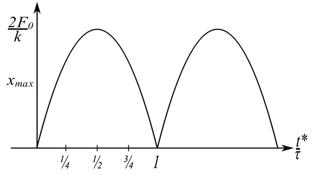
If F(t) is a rectangular pulse of length 
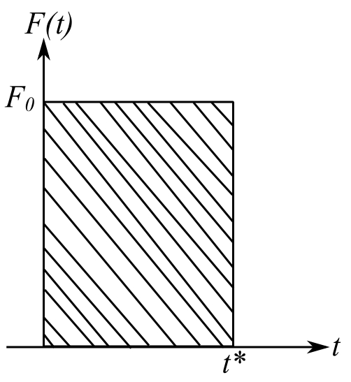
then during the pulse
![\[ x(t)=\frac{F_0}{k}(1-\cos pt) \]](https://engcourses-uofa.ca/wp-content/ql-cache/quicklatex.com-1aa3c95fcbcaa6e74528ff95bbc77d21_l3.png "Rendered by QuickLaTeX.com")
where  and after
![\[ x(t) = \frac{F_0}{k}\big[\cos p(t-t^*)-\cos pt\big] \]](https://engcourses-uofa.ca/wp-content/ql-cache/quicklatex.com-05b3cd98c11d593c3788d1a1e2060966_l3.png "Rendered by QuickLaTeX.com")
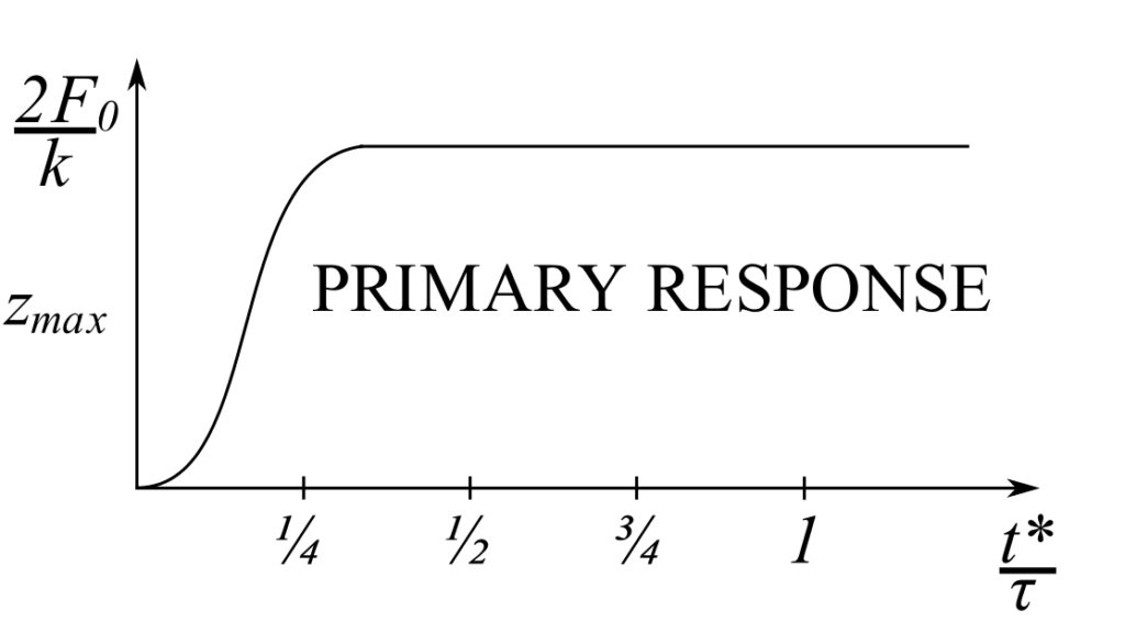
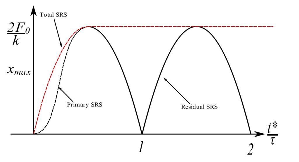
where  . Often the results are determined for the two sections (during & after) individually then combined as the primary response (during) and the residual (after pulse) response.
During the pulse
Where  for a maximum:
![\[ \frac{d}{dt}\Big(\frac{xk}{F_0}\Big)=0=p\sin pt' \]](https://engcourses-uofa.ca/wp-content/ql-cache/quicklatex.com-ac873d1667e935d1d10f9d363431bf51_l3.png "Rendered by QuickLaTeX.com")
therefore:
![\[ pt'=\pi, 2\pi, … \]](https://engcourses-uofa.ca/wp-content/ql-cache/quicklatex.com-8e160ea18c80bbd556eb996f0b5c00d1_l3.png "Rendered by QuickLaTeX.com")
![\[ t'=\frac{\pi}{p}, \frac{2\pi}{p}… \]](https://engcourses-uofa.ca/wp-content/ql-cache/quicklatex.com-b10e84b8ecf6a39197ad2c1573b58953_l3.png "Rendered by QuickLaTeX.com")
therefore up to  , the maximum is the value at the time considered as it is still increasing therefore:
![\[ x_\text{MAX} = \frac{F_0}{k}(1-\cos pt) \]](https://engcourses-uofa.ca/wp-content/ql-cache/quicklatex.com-19bbe2f9cebd13ba33b945a9a3dd0b08_l3.png "Rendered by QuickLaTeX.com")
where  . After
  the maximum is:
![\[ \begin {split} x_\text{MAX} &=\frac{F_0}{k}\Big(1-\cos\Big(\frac{p\pi}{p}\Big)\Big) \\&=2\frac{F_0}{k} \end{split} \]](https://engcourses-uofa.ca/wp-content/ql-cache/quicklatex.com-406bf8aa86a5dde9d7ed030a6b69f355_l3.png "Rendered by QuickLaTeX.com")
These results are called the primary values as they correspond to the result during the pulse.
after
![\[ \frac{kx(t)}{F_0}=\big[\cos p(t-t^*)-\cos pt\big] \]](https://engcourses-uofa.ca/wp-content/ql-cache/quicklatex.com-6a9edcd63ead5e9f91560e546e5b5120_l3.png "Rendered by QuickLaTeX.com")
where
and we find the maxima by differentiating
![\[ \frac{d}{dt}\Big(\frac{x(t)k}{F_0}\Big)=p\big[\sin p(t_1^*-t^*)-\sin pt_1^*\big]=0 \]](https://engcourses-uofa.ca/wp-content/ql-cache/quicklatex.com-8300a4d145e0ffa42a489fec44bbdf1f_l3.png "Rendered by QuickLaTeX.com")
at 
![\[ 0 = p\big[\sin pt_1 \cos pt^* - \cos pt_1 \sin pt^* -\sin pt_1\big] \]](https://engcourses-uofa.ca/wp-content/ql-cache/quicklatex.com-4f6ef80e4c526337106a0e83c61a7804_l3.png "Rendered by QuickLaTeX.com")
therefore:
![\[ \begin{split} \sin pt_1(1-\cos pt^*) &= -\sin pt^* \cos pt_1 \\ \tan pt_1 &= \frac{-\sin pt^*}{(1-\cos pt^*)} \end{split} \]](https://engcourses-uofa.ca/wp-content/ql-cache/quicklatex.com-8948307f1f54e748bb34e90014606e89_l3.png "Rendered by QuickLaTeX.com")
This value for must be inserted into the original expression to find the maximum displacement. This will require  and
and  in terms of
  and
and  .
.
therefore consider the triangle
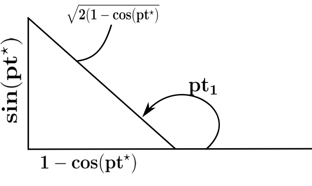
 as tan is negative], sin is negative
therefore:
![\[ \sin pt_1 = \frac{\sin pt^*}{\sqrt{2(1-\cos pt^*)}} \]](https://engcourses-uofa.ca/wp-content/ql-cache/quicklatex.com-e1ac0aced25b3690e46a1cc66ed3ab8a_l3.png "Rendered by QuickLaTeX.com")
![\[\begin{split} \cos pt_1 &= \frac{-(1-\cos pt^*)}{\sqrt{2(1-\cos pt^*)}} \\ &= -\frac{1}{\sqrt{2}} \sqrt{1-\cos pt^*} \end{split} \]](https://engcourses-uofa.ca/wp-content/ql-cache/quicklatex.com-27ace3993b2485f4aa9b4f245f103450_l3.png "Rendered by QuickLaTeX.com")
now
![\[ \begin{split} \frac{x(t_1)k}{F_0}\bigg|_{\text{MAX}} &= \cos pt^* \cos pt_1 + \sin pt^* \sin pt_1 - \cos pt_1 \\ &= -\frac{1}{\sqrt{2}}\sqrt{1-\cos pt^*}[-1+ \cos pt^*] + \frac{\sin^*2pt^*}{\sqrt{2(1-\cos pt^*}} \\ &=\frac{\frac{\sqrt{2}}{\sqrt{2}}(1-\cos pt^*)^2+\sin^*2pt^*}{\sqrt{2(1-\cos pt^*)}} \\ &= \frac{2(1-\cos pt^*)}{\sqrt{2(1-\cos pt^*)}} \\ &=\sqrt{2(1-\cos pt^*)} \\ &= 2\sin p\frac{t^*}{2} \end{split} \]](https://engcourses-uofa.ca/wp-content/ql-cache/quicklatex.com-07eae4b54125f825f76b142c6db2c16b_l3.png "Rendered by QuickLaTeX.com")
but therefore:
![\[ \frac{x(t)k}{F_0}\bigg|_{\text{MAX}} = 2\sin \frac{\pi t^*}{\tau} \]](https://engcourses-uofa.ca/wp-content/ql-cache/quicklatex.com-fe604dbe8e72847aee09c1264f20a796_l3.png "Rendered by QuickLaTeX.com")
Residual Response
The total SRS can now be determined
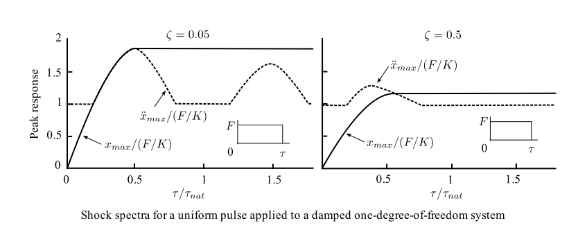
If damping is added then the magnitude can be reduced considerably. However, the calculation of the SRS must be done numerically
For cases which the pulses variation is less than one-half the period  , the overall maximum occurs after the pulse in the “free” vibration phase. As the pulse duration compared to the period becomes smaller we can approximate the response where it is the magnitude of the impulse(not the details of the shape) that matters. In the development of the theory, the response for a damped system was:
![\[x(t) = \frac{F(t^{'}) \Delta t^{'}}{mp \sqrt{1- \zeta ^{2}}} e^{-\zeta pt} \sin\big(\sqrt{1-\zeta ^{2}}pt\big)\]](https://engcourses-uofa.ca/wp-content/ql-cache/quicklatex.com-fb812da0a6ab861b16851cd72751f6d3_l3.png "Rendered by QuickLaTeX.com")
Where is the time since the impulse and for for the undamped situation
![\[x(t) = \frac{F \Delta t}{mp} \sin pt\]](https://engcourses-uofa.ca/wp-content/ql-cache/quicklatex.com-f280ad5ab1c52912a883a34251131df9_l3.png "Rendered by QuickLaTeX.com")
Where  is the impulse,
  , and the maximum displacement is:
![\[\begin{split} x_\text{MAX} &= \frac{I}{mp} \\&= \frac{I}{k} \frac{k}{mp} \\&= \frac{Ip}{k} \\&= \frac{I}{k}\frac{2 \pi}{\tau} \end{split}\]](https://engcourses-uofa.ca/wp-content/ql-cache/quicklatex.com-0b4d4e25234c30e263e8523da26a2d61_l3.png "Rendered by QuickLaTeX.com")
Consider three different impulses:
1) rectangular 2) half sine 3) triangular
1)
![\[I = F_o t^{\star}\]](https://engcourses-uofa.ca/wp-content/ql-cache/quicklatex.com-646b09c8caa7fa282c7cb3c6b8d0637d_l3.png "Rendered by QuickLaTeX.com")
Therefore,  compared to the static response due to
![\[\frac{x_\text{MAX}}{x_\text{STATIC}} = \frac{2\pi t^{\star}}{\tau}\]](https://engcourses-uofa.ca/wp-content/ql-cache/quicklatex.com-373c553b84a5945ee8bc77f5041efedd_l3.png "Rendered by QuickLaTeX.com")
2)
![\[\begin{split} I &= F_o \int_{0}^{t^{\star}} \sin \frac{\pi t}{t^{\star}} \,dt \\&= -F_o \frac{t^{\star}}{\pi} \cos\frac{\pi t}{t^{\star}} \Big|_ 0^ {t^{\star}} \\&= \frac{2F_o t^{\star}}{\pi} \end{split}\]](https://engcourses-uofa.ca/wp-content/ql-cache/quicklatex.com-583500cbc5ac28503497bba51f40e5e4_l3.png "Rendered by QuickLaTeX.com")
Therefore,
![\[\begin{split} x_\text{MAX} &= \frac{2\pi}{\tau} \frac{2F_o t^{\star}}{\pi} \\&= \frac{4 t^{\star}}{\tau} (\frac{F_o}{k}) \end{split}\]](https://engcourses-uofa.ca/wp-content/ql-cache/quicklatex.com-799f9150eb7871bc447475dac70606e4_l3.png "Rendered by QuickLaTeX.com")
3)
![\[I = \frac{F_o t^{\star}}{2}\]](https://engcourses-uofa.ca/wp-content/ql-cache/quicklatex.com-1e853410627e02888d1e2d9dd478d7a0_l3.png "Rendered by QuickLaTeX.com")
![\[x_\text{MAX} = \frac{\pi t^{\star}}{\tau} (\frac{F_o}{k})\]](https://engcourses-uofa.ca/wp-content/ql-cache/quicklatex.com-01332da77bf61fffa093e46437b1f65b_l3.png "Rendered by QuickLaTeX.com")
If the effect of damping is included then:
![\[x_\text{MAX}(t) = \Big[\frac{I}{mp \sqrt{1-\zeta ^{2}}} e\strut^{-\zeta pt} \sin\big(\sqrt{1-\zeta ^{2}}pt\big)\Big]_\text{MAX} \]](https://engcourses-uofa.ca/wp-content/ql-cache/quicklatex.com-b04a55b7c94226b717264b7e52b9c843_l3.png "Rendered by QuickLaTeX.com")
and for  we assume the maximum occurs at (or near) where
  is 1.
is 1.
Therefore  (time at
  ) is
) is  of a so-called damped period:
![\[\begin{split} \hat{t} &= \frac{\pi}{2p \sqrt{1-\zeta ^{2}}} \\& \approx \frac{\pi}{2p} \end{split}\]](https://engcourses-uofa.ca/wp-content/ql-cache/quicklatex.com-9c384f90fadcacd1d3674e65cd07e355_l3.png "Rendered by QuickLaTeX.com")
Therefore:
![\[\begin{split} x_\text{MAX} &= \frac{I}{mp} e\strut^{-\zeta p \hat{t}} \\&= \frac{I}{mp} e\strut^{-\zeta \frac{\pi}{2}} \end{split}\]](https://engcourses-uofa.ca/wp-content/ql-cache/quicklatex.com-234244550c0acc7ec664a130a6e8c1fd_l3.png "Rendered by QuickLaTeX.com")
and for  :
:
![\[x_\text{MAX} = \frac{I}{k} \frac{2\pi}{\tau} (1- \frac{\zeta \pi}{2})\]](https://engcourses-uofa.ca/wp-content/ql-cache/quicklatex.com-13be84f1bde66c8709c36c3965246883_l3.png "Rendered by QuickLaTeX.com")
and we can multiply the undamped values by  :
:
 | 0.05 | 0.10 | 0.15 | 0.20 | 0.25 | 0.3 |
 | 0.921 | 0.843 | 0.764 | 0.686 | 0.607 | 0.529 |