
Review of single and multi-degree of freedom (mdof) systems: Steady State Harmonic Response
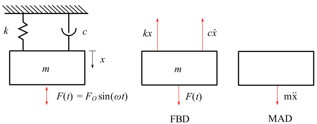
![\[ \begin{split}+\downarrow\sum F_x &= m\ddot{x} \\&= -kx-c\dot{x} + F(t) \end{split}\]](https://engcourses-uofa.ca/wp-content/ql-cache/quicklatex.com-d849b5ac40e747463f07a06959fab284_l3.png "Rendered by QuickLaTeX.com")
Therefore:
( )
) 
Therefore find solution as homogeneous solution  particular integral.
a) Homogeneous Solution:
![\[ m\ddot{x_H} + c\dot{x_H} = 0 \implies\]](https://engcourses-uofa.ca/wp-content/ql-cache/quicklatex.com-1b47f376dab8f9fa1244dd129b6bb15e_l3.png "Rendered by QuickLaTeX.com")
![\[ x_H = e^{-\zeta pt}\big[A\cos{\sqrt{1-\zeta^2}}pt+ B\sin{\sqrt{1-\zeta^2}}pt\big] \]](https://engcourses-uofa.ca/wp-content/ql-cache/quicklatex.com-8227e29fb077d30439e2eeebab40bad9_l3.png "Rendered by QuickLaTeX.com")
b) Particular integral:
Try  into
into 
![\[-m\omega^2C\sin{\omega t} - m\omega^2D\cos{\omega t} + Cc\omega\cos{\omega t}\]](https://engcourses-uofa.ca/wp-content/ql-cache/quicklatex.com-8d1a36594694fa8a65af5f0b5514c4e4_l3.png "Rendered by QuickLaTeX.com")
![\[-Dc\omega\sin{\omega t} + kC\sin{\omega t} + kD\cos{\omega t} = F_0\sin{\omega t} \]](https://engcourses-uofa.ca/wp-content/ql-cache/quicklatex.com-3ce3f0312e8e619d5d58702acccd41d7_l3.png "Rendered by QuickLaTeX.com")
Therefore:
![\[-m\omega^2C-c\omega D+kC = F_0,\]](https://engcourses-uofa.ca/wp-content/ql-cache/quicklatex.com-8335a592b9e1fdbc1c38615ba84de4d8_l3.png "Rendered by QuickLaTeX.com")
![\[-m\omega^2D+c\omega C+kD = 0\]](https://engcourses-uofa.ca/wp-content/ql-cache/quicklatex.com-bfe144161c062acfd7bd25b809ba6852_l3.png "Rendered by QuickLaTeX.com")
![\[C\Big(1-\frac{m\omega^2}{k}\Big) - \frac{c\omega}{k}D = \frac{F_0}{k}\]](https://engcourses-uofa.ca/wp-content/ql-cache/quicklatex.com-3a4dc5acd8418225f9e7ad9fcac5e5c7_l3.png "Rendered by QuickLaTeX.com")
![\[C\Big(\frac{c\omega}{k}\Big) + \Big(1-\frac{m\omega^2}{k}\Big)D = 0\]](https://engcourses-uofa.ca/wp-content/ql-cache/quicklatex.com-8259c1508388974944d78b8b16f73fc7_l3.png "Rendered by QuickLaTeX.com")
Note:
![\[ \frac{m\omega^2}{k} = \frac{\omega^2}{p^2}\]](https://engcourses-uofa.ca/wp-content/ql-cache/quicklatex.com-ed09e9c22b66677c72d2b76cb5565f6c_l3.png "Rendered by QuickLaTeX.com")
![\[ \frac{c\omega}{k} = 2\zeta\frac{\omega}{p}\]](https://engcourses-uofa.ca/wp-content/ql-cache/quicklatex.com-7119c04c05964f3a2d621148b0b47812_l3.png "Rendered by QuickLaTeX.com")
![\[ \begin{split} \implies \frac{c\omega}{k} &= \frac{c}{c_c}(2mp)\frac{\omega}{k} \\&= 2\zeta\frac{\omega}{p}\end{split}\]](https://engcourses-uofa.ca/wp-content/ql-cache/quicklatex.com-1f8e365dbc204e8a91f6f8f934349373_l3.png "Rendered by QuickLaTeX.com")
Therefore:
![\[C\Big(1-\frac{\omega^2}{p^2}\Big) - 2\zeta\frac{\omega}{p}D = 0,\]](https://engcourses-uofa.ca/wp-content/ql-cache/quicklatex.com-8aa62bd5da3c24a8ab16e0897f2afa9b_l3.png "Rendered by QuickLaTeX.com")
![\[2\zeta\frac{\omega}{p}C+\Big(1-\frac{\omega^2}{p^2}\Big)D = 0\]](https://engcourses-uofa.ca/wp-content/ql-cache/quicklatex.com-86b4902e2bf85bfdb0def482e0841217_l3.png "Rendered by QuickLaTeX.com")
Solving the above equations for C & D gives:
![\[C = \frac{\big(1-\frac{\omega^2}{p^2}\big)F_0/k}{\big(1-\frac{\omega^2}{p^2}\big)^2+\big(2\zeta\frac{\omega}{p}\big)\strut^2}\]](https://engcourses-uofa.ca/wp-content/ql-cache/quicklatex.com-fc4e6254d528971e8dd028e2a3b580c1_l3.png "Rendered by QuickLaTeX.com")
![\[D = \frac{-2\zeta\frac{\omega}{p}F_0/k}{\big(1-\frac{\omega^2}{p^2}\big)^2+\big(2\zeta\frac{\omega}{p}\big)\strut^2}\]](https://engcourses-uofa.ca/wp-content/ql-cache/quicklatex.com-b3831ebb4deb0b00e4805af35fa4915b_l3.png "Rendered by QuickLaTeX.com")
when  and
and  :
:
![\[x(t) = e^{-\zeta pt}\Big[x_o\cos{\sqrt{1-\zeta^2}}pt + \frac{v_0+\zeta px_0}{\sqrt{1-\zeta^2}}\sin{\sqrt{1-\zeta^2}}pt\Big]+C\sin{\omega t} +D\cos{\omega t}\]](https://engcourses-uofa.ca/wp-content/ql-cache/quicklatex.com-bc145f9e9aaacefbeda8243af8bf47af_l3.png "Rendered by QuickLaTeX.com")
However, if  is
is  after some time the homogeneous part will decay and the steady state solution becomes:
![\[X(_{ss}) = C\sin{\omega t} + D\cos{\omega t}\]](https://engcourses-uofa.ca/wp-content/ql-cache/quicklatex.com-6b9ca5a873c125950175c54a9a5357cd_l3.png "Rendered by QuickLaTeX.com")
If we take the special case of no clamping, the homogeneous equation is:
![\[m\ddot{x}_H + kx_H = 0\]](https://engcourses-uofa.ca/wp-content/ql-cache/quicklatex.com-588dddb5e7319cc3f391579995677705_l3.png "Rendered by QuickLaTeX.com")
![\[ x_H = A\cos{pt} + B\sin{pt}\]](https://engcourses-uofa.ca/wp-content/ql-cache/quicklatex.com-216f7fa3339977c40c9dc68147fddd0f_l3.png "Rendered by QuickLaTeX.com")
and the particular integral is
![\[x_p = C\sin{\omega t} \]](https://engcourses-uofa.ca/wp-content/ql-cache/quicklatex.com-189cad823729cc1b96a3aad346adcec4_l3.png "Rendered by QuickLaTeX.com")
Therefore:
![\[m\ddot{x}_p+kx_p = F_0\sin{\omega t}\]](https://engcourses-uofa.ca/wp-content/ql-cache/quicklatex.com-73ae9fbb795b5df7b808280964ab1ccd_l3.png "Rendered by QuickLaTeX.com")
![\[(-mC\omega^2+ck)\sin{\omega t} = F_0\sin{\omega t}\]](https://engcourses-uofa.ca/wp-content/ql-cache/quicklatex.com-d9e642ae09ae577b0927c145cfcd7f76_l3.png "Rendered by QuickLaTeX.com")
Therefore:
![\[ \begin{split} C &= \frac{F_0}{k-m\omega^2} \\&= \frac{\frac{F_0}{k}}{1-\frac{\omega^2}{p^2}} \end{split} \]](https://engcourses-uofa.ca/wp-content/ql-cache/quicklatex.com-569bb8756aa2d87e0b2241755aaa3513_l3.png "Rendered by QuickLaTeX.com")
Therefore the total solution is:
![\[ x = A\cos{pt} +B\sin{pt} + \frac{F_o/k}{1-\frac{\omega^2}{p^2}}\sin{\omega t} \]](https://engcourses-uofa.ca/wp-content/ql-cache/quicklatex.com-444fc38add88c22287625d932558ff49_l3.png "Rendered by QuickLaTeX.com")
Note that as there is no damping present that the homogeneous solution does not  as time increases.
![\[x_{ss} = C\sin{\omega t} + D\cos{\omega t}\]](https://engcourses-uofa.ca/wp-content/ql-cache/quicklatex.com-9044afed8027af6155a3b6c194bcf8cf_l3.png "Rendered by QuickLaTeX.com")
and we combine them to get:
![\[ \begin{split} x_{ss} &= \sqrt{C^2+D^2}\sin{(\omega t - \phi)} \\&= \frac{\frac{F_0}{k}}{\sqrt{\big(1-\frac{\omega^2}{p^2}\big)\strut^2+\big(2\zeta\frac{\omega}{p}\big)\strut^2}}\sin{(\omega t - \phi)} \end{split} \]](https://engcourses-uofa.ca/wp-content/ql-cache/quicklatex.com-2292ab90061ddd39e96b4550ae76bd6a_l3.png "Rendered by QuickLaTeX.com")
Where:
![\[ \tan{\phi} = \frac{2\zeta\frac{\omega}{p}}{1-\frac{\omega^2}{p^2}} \]](https://engcourses-uofa.ca/wp-content/ql-cache/quicklatex.com-1c82faa7f44443fae0202c55c5834c4b_l3.png "Rendered by QuickLaTeX.com")
This result is extremely useful in practical situations especially for controlling noise and vibration.
While this tells us the dynamic motion of the system, there is still the static deflection of the springs to be remembered. These are also related situations which are obtained by reconsideration of the fundamental equation of motion.
From the view of real situations, these are other quantities that are of interest. One of these is the force  transmitted to the supporting structure.
![\[F_T = kx +c\dot{x}\]](https://engcourses-uofa.ca/wp-content/ql-cache/quicklatex.com-a9a440d366699a3bc287eaba2d3b64c1_l3.png "Rendered by QuickLaTeX.com")
Where  is:
is:
![\[x = \frac{F_0/k}{\sqrt{\big(1-\frac{\omega^2}{p^2}\big)\strut^2+\big(2\zeta\frac{\omega}{p}\big)\strut^2}}\sin{(\omega t - \phi)}\]](https://engcourses-uofa.ca/wp-content/ql-cache/quicklatex.com-762cf5dd078c1a540c2461db71dc49c4_l3.png "Rendered by QuickLaTeX.com")
Therefore:
![\[F_T = \frac{F_0/k}{\sqrt{\big(1-\frac{\omega^2}{p^2}\big)\strut^2+\big(2\zeta\frac{\omega}{p}\big)\strut^2}} \Big[k\sin{(\omega t - \phi)} + c\omega\cos{(\omega t - \phi)}\Big]\]](https://engcourses-uofa.ca/wp-content/ql-cache/quicklatex.com-4241c69d5779c1e331f460bc88eef64d_l3.png "Rendered by QuickLaTeX.com")
and the magnitude of  (using the fact that
  ) is:
) is:
![\[\big|F_T\big| = \frac{\sqrt{k^2+(c\omega)^2}}{\sqrt{\big(1-\frac{\omega^2}{p^2}\big)\strut^2+\big(2\zeta\frac{\omega}{p}\big)\strut^2}}\]](https://engcourses-uofa.ca/wp-content/ql-cache/quicklatex.com-52323d211f376d1858294fd2aeb6f219_l3.png "Rendered by QuickLaTeX.com")
![\[\frac{|F_T|}{F_0} = \frac{\sqrt{1+\big(2\zeta\frac{\omega}{p}\big)\strut^2}}{\sqrt{\big(1-\frac{\omega^2}{p^2}\big)\strut^2+\big(2\zeta\frac{\omega}{p}\big)\strut^2}}\]](https://engcourses-uofa.ca/wp-content/ql-cache/quicklatex.com-4e7860c4fd250710d79a61a962af7267_l3.png "Rendered by QuickLaTeX.com")
A second practical situation occurs when the structure is vibrating and we wish to isolate a machine from the vibration (base excitation).
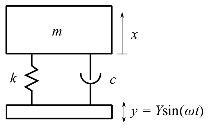
So the equation of motion is:
![\[m\ddot{x} + c\dot{x} + kx = kY\sin{\omega t}+ c\omega Y\cos{\omega t} \]](https://engcourses-uofa.ca/wp-content/ql-cache/quicklatex.com-a7236e5f2d8635c0cf03cc5bb08d3848_l3.png "Rendered by QuickLaTeX.com")
The steady state solution comes from the assumption from  :
:
![\[ \begin{split} x(t) &= C_1 \sin{\omega t} + C_2 \cos{\omega t} \\& \equiv X\sin{(\omega t - \phi)} \end{split}\]](https://engcourses-uofa.ca/wp-content/ql-cache/quicklatex.com-9c90c281528a8c21df52a46f5022f163_l3.png "Rendered by QuickLaTeX.com")
and the solution is:
![\[X = \frac{Y\sqrt{1+\big(2\zeta\frac{\omega}{p}\big)\strut^2}}{\sqrt{\big(1-\frac{\omega^2}{p^2}\big)\strut^2+\big(2\zeta\frac{\omega}{p}\big)\strut^2}}\]](https://engcourses-uofa.ca/wp-content/ql-cache/quicklatex.com-3227a74a62965497218fab937ce5690f_l3.png "Rendered by QuickLaTeX.com")
![\[ \phi = \arctan{\biggr(\frac{2\zeta\frac{\omega}{p}}{1-\frac{\omega^2}{p^2}}\biggr)}\]](https://engcourses-uofa.ca/wp-content/ql-cache/quicklatex.com-9b76e9e72e022f798218b4f658156df7_l3.png "Rendered by QuickLaTeX.com")
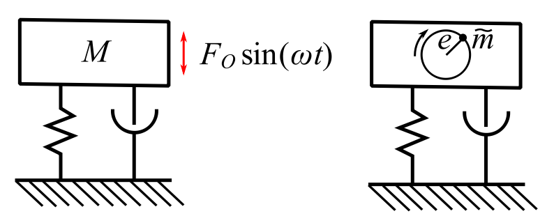
A third potential situation is essentially the original forced situation where the magnitude of the forcing function is due to rotating imbalance:
![\[F_0 = me\omega^2\]](https://engcourses-uofa.ca/wp-content/ql-cache/quicklatex.com-13ae97b87f740484094e35e2721db96a_l3.png "Rendered by QuickLaTeX.com")
Where past of the mass  , at an eccentricity
  causes the dynamic force.
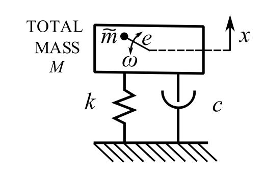
Equations of motion:
![\[ (M-\tilde{m})\ddot{x} + \tilde{m}\frac{d^2}{dt^2}(x+e\sin{\omega t}) = -kx - c\dot{x} \]](https://engcourses-uofa.ca/wp-content/ql-cache/quicklatex.com-2b5cc65d27dd14daed224e7325f011bf_l3.png "Rendered by QuickLaTeX.com")
![\[ M\ddot{x} + c\dot{x} + kx = \tilde{m}e\omega^2\sin{\omega t} \]](https://engcourses-uofa.ca/wp-content/ql-cache/quicklatex.com-bd6d7e73c8d239619d3c0021569393df_l3.png "Rendered by QuickLaTeX.com")
This looks like the previous forced case where  is replaced with
  so that:
![\[X = \frac{\tilde{m}e\omega^2}{\sqrt{(k-M\omega^2)^2+(c\omega)^2}}\]](https://engcourses-uofa.ca/wp-content/ql-cache/quicklatex.com-2c98c6e91d90b64ba5f5f4df3072e4ee_l3.png "Rendered by QuickLaTeX.com")
and reduced to non-dimensional form as:
![\[\frac{MX}{\tilde{m}e} = \frac{ \omega^2/p^2}{\sqrt{\big(1-\frac{\omega}{p}\big)\strut^2 + \big(2\zeta\frac{\omega}{p}\big)\strut^2}}\]](https://engcourses-uofa.ca/wp-content/ql-cache/quicklatex.com-d80fffe98d40e983956ecc8be2ce5c1b_l3.png "Rendered by QuickLaTeX.com")
so that the steady state solution is:
![\[x(t) = X\sin{(\omega t - \phi)}\]](https://engcourses-uofa.ca/wp-content/ql-cache/quicklatex.com-546e73af8e66d16ee9c0260cd9a6394c_l3.png "Rendered by QuickLaTeX.com")
where:
![\[ \tan{\phi} = \frac{2\zeta\frac{\omega}{p}}{1-\big(\frac{\omega}{p}\big)\strut^2}\]](https://engcourses-uofa.ca/wp-content/ql-cache/quicklatex.com-bad068431494de839b87104c1df5d4fb_l3.png "Rendered by QuickLaTeX.com")
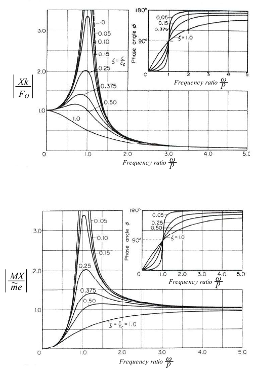
The frequency response for all these cases are summarized below.
Single Degree of Freedom Systems – Useful Relations
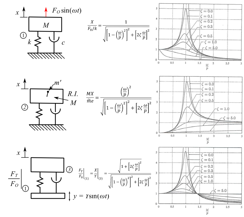
The frequency response curves are helpful in visualizing where the specific system you are analyzing lies. It must be remembered that there is a phase difference between excitation and response with the change from being nearly in phase to being nearly 180 degrees out of phase. The transition occurs near resonance ( ). For the undamped case, this means the response is undefined at
  and the response becomes:
![\[ \begin{split} \left|\frac{X}{Y}\right| &= \left|\frac{F_T}{F_0}\right| \\&= \left|\frac{X}{X_0}\right| \\& = \frac{1}{1-\frac{\omega^2}{p^2}}, \frac{\omega}{p} < 1\\& = \frac{1}{\frac{\omega^2}{p^2}-1}, \frac{\omega}{p} > 1 \end{split} \]](https://engcourses-uofa.ca/wp-content/ql-cache/quicklatex.com-b5e33d0f4d0b40bcc4fb375eac3a2ca0_l3.png "Rendered by QuickLaTeX.com")
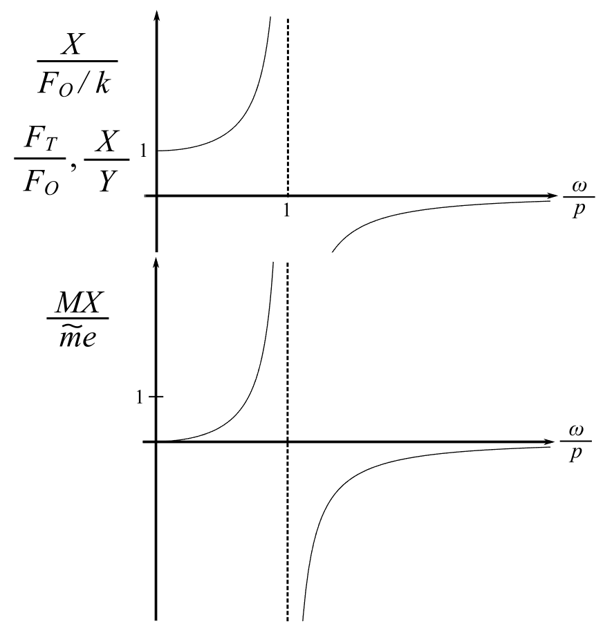
![\[\left| \frac{MX}{\tilde{m}e}\right| = \frac{\omega^2/p^2}{1-\frac{\omega^2}{p^2}}, \frac{\omega}{p} < 1\]](https://engcourses-uofa.ca/wp-content/ql-cache/quicklatex.com-4d681c21b759c2d80ef3e7eadf384de8_l3.png "Rendered by QuickLaTeX.com")
![\[\left| \frac{MX}{\tilde{m}e}\right| = \frac{\omega^2/p^2}{\frac{\omega^2}{p^2}-1}, \frac{\omega}{p} > 1\]](https://engcourses-uofa.ca/wp-content/ql-cache/quicklatex.com-bc2b3013f51c4905aa58ed07852ed6d3_l3.png "Rendered by QuickLaTeX.com")
The results for the steady state forced single degree of freedom systems are usually present in the form of graphs showing various non-dimensional parameters. Because of the technical importance of these results, it is necessary to understand the differences between these representations. Two of the most useful are given by the expressions for displacement of the mass:
![\[\left|\frac{X}{X_0}\right| = \left|\frac{1}{\sqrt{\big(1-\frac{\omega^2}{p^2}\big)\strut^2 + \big(2\zeta\frac{\omega}{p}\big)\strut^2}}\right|(A)\]](https://engcourses-uofa.ca/wp-content/ql-cache/quicklatex.com-d83a8650e91e3320021371fea5b46395_l3.png "Rendered by QuickLaTeX.com")
And the displacement of the main mass in the case of rotating imbalance:
![\[\left| \frac{MX}{\tilde{m}e}\right| = \left|\frac{\omega^2/p^2}{\sqrt{\big(1-\frac{\omega^2}{p^2}\big)\strut^2 + \big(2\zeta\frac{\omega}{p}\big)\strut^2}}\right|(B)\]](https://engcourses-uofa.ca/wp-content/ql-cache/quicklatex.com-4e56a0a2d109ad77e24016dea695f848_l3.png "Rendered by QuickLaTeX.com")
a) Show that (B) can be derived from (A) for the special case in which the forcing function is due to rotating imbalance
b) For the undamped case determine the result of (A) and (B) both below and above resonance
a) Special cases for rotating imbalance:
![\[X_0 = \frac{F_0}{k}\]](https://engcourses-uofa.ca/wp-content/ql-cache/quicklatex.com-9ae660b10b8223ff5939e5ea399cfb1d_l3.png "Rendered by QuickLaTeX.com")
If  :
:
![\[ X_0 = \frac{\tilde{m}e\omega^2}{k}\]](https://engcourses-uofa.ca/wp-content/ql-cache/quicklatex.com-3ca57bbd20f4281834a21fe461bff4eb_l3.png "Rendered by QuickLaTeX.com")
![\[\frac{xk}{\tilde{m}e\omega^2} = \frac{1}{\sqrt{\big(1-\frac{\omega^2}{p^2}\big)\strut^2 + \big(2\zeta\frac{\omega}{p}\big)\strut^2}}\]](https://engcourses-uofa.ca/wp-content/ql-cache/quicklatex.com-69b0da9ed46a26370d58692350d63938_l3.png "Rendered by QuickLaTeX.com")
![\[\frac{Mxk}{M\tilde{m}e\omega^2} = \frac{xp^2M}{\tilde{m}e\omega^2}\]](https://engcourses-uofa.ca/wp-content/ql-cache/quicklatex.com-bba21eeb6da08d5bd9fd7993ca726ac8_l3.png "Rendered by QuickLaTeX.com")
Note:  includes the imbalanced mass
b)  for
for  is:
is:
![\[\begin{split} \left|\frac{X}{X_0}\right| &= \left|\frac{1}{\sqrt{1-\frac{\omega^2}{p^2}}}\right|, \frac{\omega}{p}\neq 1 \\&= \frac{1}{1-\frac{\omega^2}{p^2}}, \frac{\omega}{p}< 1 \\&= \frac{1}{\frac{\omega^2}{p^2}-1}, \frac{\omega}{p}> 1\end{split}\]](https://engcourses-uofa.ca/wp-content/ql-cache/quicklatex.com-f241ed3d273462b67e1bd9bd8aabe8e4_l3.png "Rendered by QuickLaTeX.com")
![\[\begin{split} \left| \frac{MX}{\tilde{m}e}\right|&= \left|\frac{\omega^2/p^2}{\sqrt{1-\frac{\omega^2}{p^2}}}\right|, \frac{\omega}{p}\neq 1 \\&= \frac{\omega^2/p^2}{1-\frac{\omega^2}{p^2}}, \frac{\omega}{p} < 1 \\&= \frac{\omega^2/p^2}{\frac{\omega^2}{p^2}-1}, \frac{\omega}{p} > 1 \end{split}\]](https://engcourses-uofa.ca/wp-content/ql-cache/quicklatex.com-74fe9b14bedbf974ebcac3304b04ccef_l3.png "Rendered by QuickLaTeX.com")
There are two important physical phenomena that are easily illustrated using the forced undamped SDOF system as we approach resonance. The entire solution:
![\[x(t) = C_1\cos pt + C_2 \sin pt + \frac{F_o}{k}\frac{\sin \omega t}{1-\frac{\omega^2}{p^2}}\]](https://engcourses-uofa.ca/wp-content/ql-cache/quicklatex.com-53026210570d16a4c53fd70bca192799_l3.png "Rendered by QuickLaTeX.com")
Consider the case  ,
,  (starting with no motion).
From the first of these  and
and
![\[ \dot{x}(t) = C_2p\cos pt+\frac{F_o}{k}\frac{1}{1-\frac{\omega^2}{p^2}} \omega \cos \omega t \]](https://engcourses-uofa.ca/wp-content/ql-cache/quicklatex.com-e5a764e7693d1421231b5e71e97ae8ab_l3.png "Rendered by QuickLaTeX.com")
Therefore at t = 0:
![\[ \begin{split} C_2 &= \frac{-F_o}{k}\frac{\frac{\omega}{p}}{1-\frac{\omega^2}{p^2}} \\&=\frac{-F_o}{k}\frac{\omega p}{p^2-\omega^2} \end{split} \]](https://engcourses-uofa.ca/wp-content/ql-cache/quicklatex.com-f46f786dbddec8d259300ce43b0e9a52_l3.png "Rendered by QuickLaTeX.com")
![\[ x(t) = \frac{F_o}{k}\frac{p^2}{p^2-\omega^2}\big[\sin \omega t-\frac{\omega}{p}\cos pt\big] \]](https://engcourses-uofa.ca/wp-content/ql-cache/quicklatex.com-3c5aab0718a8cada447031ab9a7ba81f_l3.png "Rendered by QuickLaTeX.com")
If  , where
  is small compared to
  or
or  , then:
![\[ x(t) = \frac{F_op^2}{k}\frac{1}{p^2-\omega^2}\big[\sin \omega t - \sin pt\big] \]](https://engcourses-uofa.ca/wp-content/ql-cache/quicklatex.com-f14b25ddb111b42801a033ea414411c7_l3.png "Rendered by QuickLaTeX.com")
( ), therefore:
![\[ x = 2\frac{F_op^2}{k(p^2-\omega^2)}\cos \omega t\sin\Delta t \]](https://engcourses-uofa.ca/wp-content/ql-cache/quicklatex.com-d741c90533db6ca375ed8c8be534cb67_l3.png "Rendered by QuickLaTeX.com")
![\[ \begin{split} p^2-\omega^2 & = (2\Delta + \omega)^2 - \omega^2 \nonumber \\ & = 4\Delta+4\Delta \omega \nonumber \end{split} \]](https://engcourses-uofa.ca/wp-content/ql-cache/quicklatex.com-04aadf4747aa867f09dbd98d6a4d4d7e_l3.png "Rendered by QuickLaTeX.com")
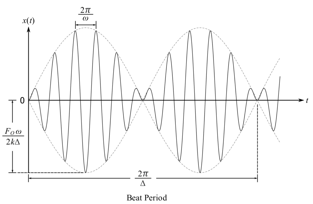
Therefore:
![\[ x = \frac{-F_o}{2k\Delta}\cos\omega t \sin\Delta t \]](https://engcourses-uofa.ca/wp-content/ql-cache/quicklatex.com-708b0a91399f46329ccf813464508c60_l3.png "Rendered by QuickLaTeX.com")
This expression can be considered as representing a vibration with period  that has a slowly varying amplitude equal to
  , (
, ( has a much longer period than
  )
)
While the original solution to the forced undamped differential equation is not valid at  , it is of value to consider what happens at
  0 for the displacement. Using L’Hospital’s rule for the following limit:
![\[ \begin{split} \lim_{\Delta \to 0} \biggr(\frac{-F_o\omega}{2k}\cos\omega t \frac{\sin \Delta t}{\Delta} \biggr) &= \frac{-F_o \omega}{2k} \cos(\omega t) t\cos \Delta t \\&= \frac{-F_o\omega}{2k}t\cos\omega t \end{split} \]](https://engcourses-uofa.ca/wp-content/ql-cache/quicklatex.com-97aa129a7fecf48d71d3894dd875bed6_l3.png "Rendered by QuickLaTeX.com")
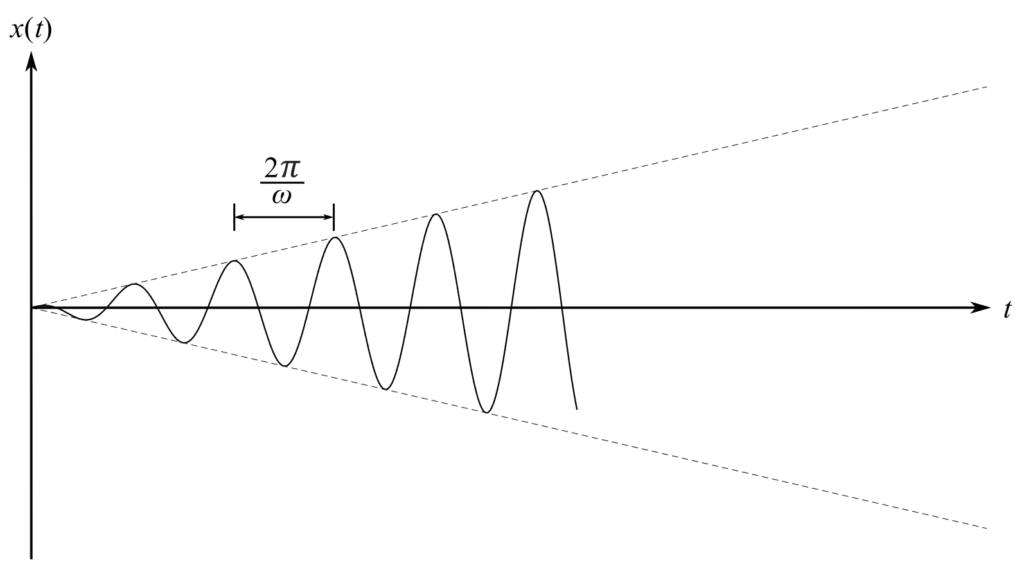
The amplitude of vibration increases indefinitely with time and the infinite amplitude is in the steady state. This means that to operate the system it is important to move through resonance as quickly as possible so that the amplitude does not “build up”.