
Advanced Dynamics and Vibrations: Modal analysis of mdof systems with generalized coordinates, semi-definite systems, repeated roots
Introduction to Normal Mode Analysis
Our analysis of MDOF systems has shown that regardless of the coordinates used that there are specific properties of the system(natural frequencies, mode shapes) that do not depend on our choices. These properties can be used to uncouple the equations of motion into  equations that can be easily solved and then transformed back to the original coordinates which are the most useful form to use the results. The process uses the modal shapes, in the form of vectors, to build a modal matrix. Consider the modal vectors
  . The modal matrix is formed by making these vectors the columns in the matrix:
![\[ [u] = \big[ \{u\}_1,\{u\}_2\dots \{u\}_m \big] \]](https://engcourses-uofa.ca/wp-content/ql-cache/quicklatex.com-c09185747bd1f79c25c763d274ecf43b_l3.png "Rendered by QuickLaTeX.com")
but instead of using ![[u]](https://engcourses-uofa.ca/wp-content/ql-cache/quicklatex.com-035b4761ef192ed27d1ab30473aafeaf_l3.png "Rendered by QuickLaTeX.com") we normalize it to
we normalize it to ![[\mu]](https://engcourses-uofa.ca/wp-content/ql-cache/quicklatex.com-9c5362d384456e76e359ae6e37e63a7a_l3.png "Rendered by QuickLaTeX.com") using the mass matrix so that:
using the mass matrix so that:
![\[ [\mu]^T[m][\mu ] = [I] \]](https://engcourses-uofa.ca/wp-content/ql-cache/quicklatex.com-a15dbf76c3331cb2b5ccdb3fd71b7daf_l3.png "Rendered by QuickLaTeX.com")
or
![\[ [\mu]_i^T[m][\mu ]_i = 1 \]](https://engcourses-uofa.ca/wp-content/ql-cache/quicklatex.com-8500f89004962a34d948d8aa4d3e67b2_l3.png "Rendered by QuickLaTeX.com")
NOTE:
![\[ [\mu]_i^T[m][\mu]_j = 0,\ i \ne j\]](https://engcourses-uofa.ca/wp-content/ql-cache/quicklatex.com-10b0af7ae12a96a4dd5406dde4307a15_l3.png "Rendered by QuickLaTeX.com")
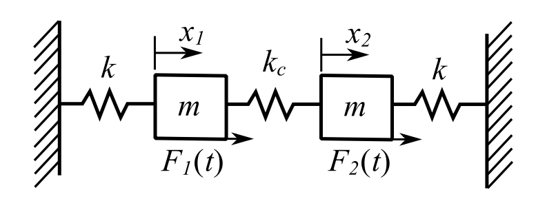
To start, consider the undamped forced 2DOF system:
![\[ \{x\} = \{X\}\sin{\omega t} \]](https://engcourses-uofa.ca/wp-content/ql-cache/quicklatex.com-0f7dafc7a2c9f62d279bf5a122d45bff_l3.png "Rendered by QuickLaTeX.com")
Therefore:
![\[ \begin{bmatrix} m & 0 \\ 0 & m \end{bmatrix} \begin{Bmatrix} \ddot{x}_1 \\ \ddot x_2 \end{Bmatrix} + \begin{bmatrix} k+ k_c & - k_c \\ -k_c & k+ k_c \end{bmatrix} \begin{Bmatrix} x_1 \\ x_2 \end{Bmatrix} = \begin{Bmatrix} F_1(t) \\ F_2(t) \end{Bmatrix} \]](https://engcourses-uofa.ca/wp-content/ql-cache/quicklatex.com-88ad10261d31193092312d655a482b7f_l3.png "Rendered by QuickLaTeX.com")
![\[ p_{1,2}^2 = \frac{k}{m},\ \frac{k+2k_c}{m} \]](https://engcourses-uofa.ca/wp-content/ql-cache/quicklatex.com-267f7edb91306ce5c3c21772a94c80d1_l3.png "Rendered by QuickLaTeX.com")
![\[ \{u\}_1 = \begin{Bmatrix} X_1 \\ X_2 \end{Bmatrix}^{(1)} = \begin{Bmatrix} 1 \\ 1 \end{Bmatrix} \]](https://engcourses-uofa.ca/wp-content/ql-cache/quicklatex.com-1dbd1c6546a407321dd6e735b5b724d5_l3.png "Rendered by QuickLaTeX.com")
![\[ \{u\}_2 = \begin{Bmatrix} X_1 \\ X_2 \end{Bmatrix}^{(2)} = \begin{Bmatrix} 1 \\ -1 \end{Bmatrix} \]](https://engcourses-uofa.ca/wp-content/ql-cache/quicklatex.com-d125209a68b0cf541ecc2c67fbcd4dbc_l3.png "Rendered by QuickLaTeX.com")
Normalize  and
and  using
using ![\alpha_i^2\{u\}_i^T[m]\{u\}_i = 1](https://engcourses-uofa.ca/wp-content/ql-cache/quicklatex.com-9c5dcf7ace6c6f48a454ad50b3676fd0_l3.png "Rendered by QuickLaTeX.com") where
where  . Therefore:
![\[ \alpha_1^2 \begin{Bmatrix} 1 & 1 \end{Bmatrix} \begin{bmatrix} m & 0 \\ 0 & m \end{bmatrix} \begin{Bmatrix} 1 \\ 1 \end{Bmatrix} = 1 \]](https://engcourses-uofa.ca/wp-content/ql-cache/quicklatex.com-c1c7edbec9c73f30b92585b16ca79c6f_l3.png "Rendered by QuickLaTeX.com")
![\[ \alpha_1 = \frac{1}{\sqrt{2m}} \]](https://engcourses-uofa.ca/wp-content/ql-cache/quicklatex.com-b0092ba1699ec49fc735cf51fddcbba1_l3.png "Rendered by QuickLaTeX.com")
![\[ \alpha_2^2 \begin{Bmatrix} 1 & -1 \end{Bmatrix} \begin{bmatrix} m & 0 \\ 0 & m \end{bmatrix} \begin{Bmatrix} 1 \\ -1 \end{Bmatrix} = 1 \]](https://engcourses-uofa.ca/wp-content/ql-cache/quicklatex.com-3d70e64d13a86f51f871c0052d6576b4_l3.png "Rendered by QuickLaTeX.com")
![\[ \alpha_2 = \frac{1}{\sqrt{2m}} \]](https://engcourses-uofa.ca/wp-content/ql-cache/quicklatex.com-4c386996fd02a725cb8dd707c28ea77e_l3.png "Rendered by QuickLaTeX.com")
Therefore:
![\[ \{\mu \}^{(1)} = \frac{1}{\sqrt{2m}}\begin{Bmatrix} 1\\ 1 \end{Bmatrix} \]](https://engcourses-uofa.ca/wp-content/ql-cache/quicklatex.com-a7b122a0bc3acb5e23e045349cdca164_l3.png "Rendered by QuickLaTeX.com")
![\[ \{\mu \}^{(2)} = \frac{1}{\sqrt{2m}}\begin{Bmatrix} 1\\ -1 \end{Bmatrix} \]](https://engcourses-uofa.ca/wp-content/ql-cache/quicklatex.com-95d6e9f040bfa95e527d76c8d897b781_l3.png "Rendered by QuickLaTeX.com")
NOTE Orthogonality:
![\[ \begin{Bmatrix} 1 & 1 \end{Bmatrix} \begin{bmatrix} m & 0 \\ 0 & m \end{bmatrix} \begin{Bmatrix} 1 \\ -1 \end{Bmatrix} = \begin{Bmatrix} 1 & 1 \end{Bmatrix} \begin{Bmatrix} m \\ -m\end{Bmatrix} = 0\]](https://engcourses-uofa.ca/wp-content/ql-cache/quicklatex.com-8fc787051adab80d517efb2a4b6b789b_l3.png "Rendered by QuickLaTeX.com")
![\[ \begin{Bmatrix} 1 & -1 \end{Bmatrix} \begin{bmatrix} k + k_c & -k_c \\ -k_c & k+k_c \end{bmatrix} \begin{Bmatrix} 1 \\ 1 \end{Bmatrix} = 0 \]](https://engcourses-uofa.ca/wp-content/ql-cache/quicklatex.com-48e4bf2fc4b871efc3ac898b7765a464_l3.png "Rendered by QuickLaTeX.com")
Modal vectors are orthogonal with respect to ![[m]](https://engcourses-uofa.ca/wp-content/ql-cache/quicklatex.com-04fd13cfffa1864cf42c2e3f94f29dcb_l3.png "Rendered by QuickLaTeX.com") or
or ![[k]](https://engcourses-uofa.ca/wp-content/ql-cache/quicklatex.com-36cac14b0049be6314d64ed283924d13_l3.png "Rendered by QuickLaTeX.com") . Thefore the modal matrix is:
. Thefore the modal matrix is:
![\[ [\mu ] = \frac{1}{\sqrt{2m}} \begin{bmatrix} 1 & 1 \\ 1 & -1 \end{bmatrix} \]](https://engcourses-uofa.ca/wp-content/ql-cache/quicklatex.com-b33b1484dd759159eb282c194b9c6f2d_l3.png "Rendered by QuickLaTeX.com")
![\[ [\mu ]^{-1} = \sqrt{\frac{m}{2}} \begin{bmatrix} -1 & -1 \\ -1 & 1 \end{bmatrix} \]](https://engcourses-uofa.ca/wp-content/ql-cache/quicklatex.com-cc18b05b293f0031a0c50af5b8ad4866_l3.png "Rendered by QuickLaTeX.com")
Now transform the equations of motion using ![[\mu ]](https://engcourses-uofa.ca/wp-content/ql-cache/quicklatex.com-361ba9fa1ff66077298e4e9225144994_l3.png "Rendered by QuickLaTeX.com") by setting
by setting ![\{x\} = [\mu] \{\eta\}](https://engcourses-uofa.ca/wp-content/ql-cache/quicklatex.com-217056491c2090d001d0f2fdf86da885_l3.png "Rendered by QuickLaTeX.com") then
then ![\{\ddot{x} \} = [\mu][\ddot{\eta}]](https://engcourses-uofa.ca/wp-content/ql-cache/quicklatex.com-8359b0e4d036a1313fa2fc87906a5f89_l3.png "Rendered by QuickLaTeX.com") .
.
![\[ [\mu]^T[m][\mu ] &= \frac{1}{2m} \begin{bmatrix} 1 & 1 \\ 1 & -1 \end{bmatrix} \begin{bmatrix} m & 0 \\ 0 & m \end{bmatrix} \begin{bmatrix} 1 & 1 \\ 1 & -1 \end{bmatrix} = \begin{bmatrix} 1 & 0 \\ 0 & 1\end{bmatrix}\]](https://engcourses-uofa.ca/wp-content/ql-cache/quicklatex.com-97843bf2e471d9d639a34bfeaa8b422f_l3.png "Rendered by QuickLaTeX.com")
![\[[\mu]^T[k][\mu] = \begin{bmatrix} \frac{k}{m} & 0 \\ 0 & \frac{k+2k_c}{m} \end{bmatrix} \]](https://engcourses-uofa.ca/wp-content/ql-cache/quicklatex.com-d68f18f65ffd192b7f989e6fd9614acc_l3.png "Rendered by QuickLaTeX.com")
Now multiply the equations of motion by ![[\mu ] ^T](https://engcourses-uofa.ca/wp-content/ql-cache/quicklatex.com-7f8d11187d48858abc0e8c3e9f064b8c_l3.png "Rendered by QuickLaTeX.com") to get:
to get:
![\[\mu ] ^T[m][\mu]\{ \ddot{\eta }\} + [\mu]^T[k][\mu ]\{ \eta \} = [\mu ]^T \{F \} \]](https://engcourses-uofa.ca/wp-content/ql-cache/quicklatex.com-4e5dac22d2fc3506a2ae8453c7a5e647_l3.png "Rendered by QuickLaTeX.com")
Therefore, the transformed equations become

Where

We can now solve this set of uncoupled SDOF equations for the free, transient on steady-state conditions. In the transformed state the stiffness matrix is now the matrix of natural frequencies:

After solving we transform back to the original condition.
Normal analysis of MDOF systems
The equations of motion for viscously damped MDOF systems are in general
![\[ [m] \{\ddot{x}\} + [c] \{\dot{x}\} + [k] \{x\} = \{F(t)\}\]](https://engcourses-uofa.ca/wp-content/ql-cache/quicklatex.com-2e00885cd0f87242c9c24f81287a4cf8_l3.png "Rendered by QuickLaTeX.com")
For up to 2 DOF we can easily use a complex analysis (transform methods). However for larger system we often use modal analysis.
In this approach we start with the homogeneous equations and we will also start with the undamped case. (We will return to it later!) Therefore,
![\[ [m] \{ \ddot{x} \} + [k] \{x \} = \{0\}\]](https://engcourses-uofa.ca/wp-content/ql-cache/quicklatex.com-0b68f473c7f62071aa3246dd57f63ec3_l3.png "Rendered by QuickLaTeX.com")
We look for so-called synchronous motions SSHM (Simultaneous Simple Harmonic motion) by assuming
![\[\{x\} = \{u\} \sin (pt+\phi) \]](https://engcourses-uofa.ca/wp-content/ql-cache/quicklatex.com-88f0f1ccf212b13bbf6d7883e7dcc83e_l3.png "Rendered by QuickLaTeX.com")
or
![\[\{x\} = \{u\} \cos (pt-\psi)\]](https://engcourses-uofa.ca/wp-content/ql-cache/quicklatex.com-939371fc27023a50228cff42168b302c_l3.png "Rendered by QuickLaTeX.com")
and get
![\[p^{2}[m]\{u\} = [k]\{u\}\]](https://engcourses-uofa.ca/wp-content/ql-cache/quicklatex.com-8f60c184452824a7231c0e6c76364f52_l3.png "Rendered by QuickLaTeX.com")
This is true for only special  say
say  and special
  associated with
We can find the & the within a multiplicative constant. Each  and its associated is called a mode.
If the are distinct then we can easily show that the are orthogonal to one another in some sense. To see this consider the two modes say  &
&  , then
![\[[k]\{u\}_{i} = p_{i}^{2}[m]\{u\}_{i}\]](https://engcourses-uofa.ca/wp-content/ql-cache/quicklatex.com-c36b2936b178aaf04b405f3086ede93b_l3.png "Rendered by QuickLaTeX.com")
![\[[k]\{u\}_{j} = p_{j}^{2}[m]\{u\}_{j}\]](https://engcourses-uofa.ca/wp-content/ql-cache/quicklatex.com-86f35525d579660af324cc2e7c7ea212_l3.png "Rendered by QuickLaTeX.com")
Multiply the first by 
![\[\{u\}_{j}^{T} [k] \{u\}_{i} = p_{i}^{2} \{u\}_{j}^{T} [m]\{u\}_{i}\]](https://engcourses-uofa.ca/wp-content/ql-cache/quicklatex.com-04fa0aba69636e1b14a53ff00da657e9_l3.png "Rendered by QuickLaTeX.com")
and the second by 
![\[\{u\}_{i}^{T} [k] \{u\}_{j} = p_{j}^{2} \{u\}_{i}^{T} [m]\{u\}_{j}\]](https://engcourses-uofa.ca/wp-content/ql-cache/quicklatex.com-c36d9e0544ca986759b9d976f3de138b_l3.png "Rendered by QuickLaTeX.com")
Since we can transpose the first equation so that the left hand side are the same. It suggests that
![\[\{u\}_{j}^{T} [k] \{u\}_{i} = \{u\}_{j}^{T} [m] \{u\}_{j} = 0\]](https://engcourses-uofa.ca/wp-content/ql-cache/quicklatex.com-6430f11b443a60a1380a618f7f9f3b9f_l3.png "Rendered by QuickLaTeX.com")
Therefore, the modal vector are orthogonal with respect to the mass and stiffness matrices.
These eigenvectors form a linearly independent set i.e. any motion of the system can be thought of as a linear combination of these modes. Physically this implies that any motion can be thought of as a superposition of these normal modes.
Linear independence means that we cannot write any vector as a combination of the others. If they were linearly dependent there should be some way to combine them to produce one from the others. This means there should be:
![\[\alpha _{1} \{u\}_{1} + \alpha _{2} \{u\}_{2} + \alpha _{3} \{u\}_{3} + ... = 0\]](https://engcourses-uofa.ca/wp-content/ql-cache/quicklatex.com-ef605ddc8c761603e324537ca45eecc2_l3.png "Rendered by QuickLaTeX.com")
But if we premultiply this equation by ![\{u\}_{s} [m]](https://engcourses-uofa.ca/wp-content/ql-cache/quicklatex.com-5a22bcd3571db3b30449d92cc5175fc0_l3.png "Rendered by QuickLaTeX.com") we get:
we get:
![\[ \sum_{r=1}^{n}\alpha _{r} \{u\}_{s} [m] \{u\}_{r} = 0 \]](https://engcourses-uofa.ca/wp-content/ql-cache/quicklatex.com-323b3fc04bb20cf99876673ca21fabb2_l3.png "Rendered by QuickLaTeX.com")
but all the terms are zero (orthogonality) except for  and therefore
  . The same is true for each term therefore
As a result any motion can be written as a linear combination of the modal vectors. They are a set of basis vectors in the same way as  are for
  positions. Therefore,
![\[\{u\} = \alpha _{1} \{u\}_{1} + \alpha _{2} \{u\}_{2} + \alpha _{3} \{u\}_{3} + ...\]](https://engcourses-uofa.ca/wp-content/ql-cache/quicklatex.com-29a4b4b8bb6dcecfcad51412c5dcf264_l3.png "Rendered by QuickLaTeX.com")
Where  is the modal participation factor and
![\[\alpha _{r} = \{u\}_{r}^{T} [m] \{u\}\]](https://engcourses-uofa.ca/wp-content/ql-cache/quicklatex.com-2212a8530c58f69337eea620d4af0b0f_l3.png "Rendered by QuickLaTeX.com")
This is called the expansion theorem in vibration where the  are functions of time.
It turns out that if we have repeated eigenvalue we can still find a set of eigenvectors that span the system.
We can use these properties of the system to solve these equations in general. The process uses the modal vectors put together in a so-called modal matrix. Before starting we will normalize the modal vectors into  as they are only known to within a multiplicative constant.
The normalization is:
![\[\{\mu\}_{i} [m] \{\mu\}_{i}^{T} = 1\]](https://engcourses-uofa.ca/wp-content/ql-cache/quicklatex.com-c056d0221ac8d3bb714395d64da6bacf_l3.png "Rendered by QuickLaTeX.com")
Therefore,
![\[\{\mu\}_{i} = \alpha _{i} \{u\}_{i}\]](https://engcourses-uofa.ca/wp-content/ql-cache/quicklatex.com-0b8070ecb2ed5f24ae27fe6c157540e6_l3.png "Rendered by QuickLaTeX.com")
Now form the modal matrix
![\[[\mu] = [\{u\}_{1} \{u\}_{2} \cdot \cdot \cdot \{u\}_{n}]\]](https://engcourses-uofa.ca/wp-content/ql-cache/quicklatex.com-661b230335b395a449cdc5517c649fd2_l3.png "Rendered by QuickLaTeX.com")
Then
![\[[\mu]^{T} [m] [\mu] = [I]\]](https://engcourses-uofa.ca/wp-content/ql-cache/quicklatex.com-3bef1af42a25091a5e51fb851874d78e_l3.png "Rendered by QuickLaTeX.com")
Therefore
![\[[\mu]^{T} [k] [\mu] = [p^{2}]\]](https://engcourses-uofa.ca/wp-content/ql-cache/quicklatex.com-96e135a3b97441abb12c4fca9d420427_l3.png "Rendered by QuickLaTeX.com")
Now to solve the original system we transform the equations to a set of generalized coordinates. That is we set:
![\[\{x(t)\} = [\mu] \{\eta (t)\}\]](https://engcourses-uofa.ca/wp-content/ql-cache/quicklatex.com-dfbda6cf56e19232d554b99d2c974956_l3.png "Rendered by QuickLaTeX.com")
![\[\{\ddot{x} (t)\} = [\mu] \{\ddot{\eta} (t)\}\]](https://engcourses-uofa.ca/wp-content/ql-cache/quicklatex.com-54e98f4f40569a9a46092eada7a40a60_l3.png "Rendered by QuickLaTeX.com")
putting this into the original set of equation gives:
![\[[m][\mu]\{\ddot{\eta}(t)\} + [k][\mu]\{\eta (t)\} = \{F(t)\}\]](https://engcourses-uofa.ca/wp-content/ql-cache/quicklatex.com-3edbbe5146026faa237fb9af9d52af51_l3.png "Rendered by QuickLaTeX.com")
now premultiply by ![[\mu]^{T}](https://engcourses-uofa.ca/wp-content/ql-cache/quicklatex.com-52076224ca118dfcad6e692a6a28e2a4_l3.png "Rendered by QuickLaTeX.com")
![\[\{\ddot{\eta} (t)\} + [p^{2}]\{\eta (t)\} = [\mu]^{T} \{F(t)\} = \{N(t)\}\]](https://engcourses-uofa.ca/wp-content/ql-cache/quicklatex.com-1ba630d879564dc2ffb158c9993ee636_l3.png "Rendered by QuickLaTeX.com")
This uncouples the equations so that each looks like:
![\[\ddot{\eta}_{r}(t) + p^{2}_{r} \eta _{r} (t) = N_{r} (t)\]](https://engcourses-uofa.ca/wp-content/ql-cache/quicklatex.com-378abc7d723ef19a0e9fb3cac63c18ff_l3.png "Rendered by QuickLaTeX.com")
The general solution of this equation is:
![\[\eta _{r} (t) = \frac{1}{p_{r}} \int_{0}^{t} N_{r} (\tau) \sin p(t - \tau) \,d\tau + \eta _{r} (0) \cos p_{r}t + \frac{\dot{\eta}_{r}(0)}{p_{r}} \sin p_{r} t\]](https://engcourses-uofa.ca/wp-content/ql-cache/quicklatex.com-2b57fb3b084443d886f946616e35f55d_l3.png "Rendered by QuickLaTeX.com")
We can then transform the solution back to the original coordinates using:
![\[\begin{split} \{x(t)\} &= [\mu] \{\eta (t)\} \\&= \sum_{r=1}^{n} \{\mu\}_{r} \eta _{r} (t) \end{split}\]](https://engcourses-uofa.ca/wp-content/ql-cache/quicklatex.com-18fee1cfe8593a42fb464817009eee39_l3.png "Rendered by QuickLaTeX.com")
This expression contains the initial conditions in the transformed coordinates and are related to the original values by:
![\[\{x(0)\} = [\mu] \{\eta (0)\}\]](https://engcourses-uofa.ca/wp-content/ql-cache/quicklatex.com-29d56b34d6d199a25e8410f2bb556165_l3.png "Rendered by QuickLaTeX.com")
![\[\{\dot{x} (0)\} = [\mu] \{\dot{\eta} (0)\}\]](https://engcourses-uofa.ca/wp-content/ql-cache/quicklatex.com-a14cb4abb057e1b8d3538e2527fc688c_l3.png "Rendered by QuickLaTeX.com")
We can also solve the steady-state forced problem by simply considering the particular integral instead of the total solution.
Summary (Free Vibration)
We have been considering the solution of
![\[[m]\{\ddot{x}\} + [k]\{x\} = \{0\} \qquad (\star)\]](https://engcourses-uofa.ca/wp-content/ql-cache/quicklatex.com-2b3f4d7ed057f2ab79d02d9732240aba_l3.png "Rendered by QuickLaTeX.com")
Where we transform the equation using
![\[\begin{split}\{x(t)\} &= [\mu] \{\eta(t)\} \\ \{\ddot{x}(t)\} &= [\mu]\{\ddot{\eta}(t)\}\end{split}\]](https://engcourses-uofa.ca/wp-content/ql-cache/quicklatex.com-f5f9259a54f8669a5b7d89217bc43d59_l3.png "Rendered by QuickLaTeX.com")
If we premultiply by and substitute into  we get:
![\[\{0\} = [\mu]^{T}[m][\mu] \{\ddot{\eta}(t)\} + [\mu]^{T}[k][\mu] \{\eta (t)\}\]](https://engcourses-uofa.ca/wp-content/ql-cache/quicklatex.com-535f7eaad5bf679894337c886fc2e853_l3.png "Rendered by QuickLaTeX.com")
but
![\[[\mu]^{T}[m][\mu] = [I]\]](https://engcourses-uofa.ca/wp-content/ql-cache/quicklatex.com-f6912c44e41b416738f1ec1202836909_l3.png "Rendered by QuickLaTeX.com")
![\[[\mu]^{T}[k][\mu] = [p^{2}]\]](https://engcourses-uofa.ca/wp-content/ql-cache/quicklatex.com-cadb27d501c5724f5111b1fb29466d13_l3.png "Rendered by QuickLaTeX.com")
Therefore
![\[\{\ddot{\eta}(t)\} +[p^{2}] \{\eta (t)\} = \{0\} \qquad (\star \star)\]](https://engcourses-uofa.ca/wp-content/ql-cache/quicklatex.com-5164357e2fab5b5be8e5ce241058afbe_l3.png "Rendered by QuickLaTeX.com")
The solution to these equation  is
is
![\[\eta _{r} (t) = C_{r} \cos (p_{r}t - \phi _{r})\]](https://engcourses-uofa.ca/wp-content/ql-cache/quicklatex.com-fd8600a48898ea95c24dcebc39200bf3_l3.png "Rendered by QuickLaTeX.com")
Where  &
&  are constants, therefore
![\[\begin{split} \{x(t)\} &= [\mu] \{\eta (t)\} \\&= \sum_{r=1}^{n} \eta _{r} (t) \{\mu\}_{r} \\&= \sum_{r=1}^{n} C_{r} \{\mu\}_{r} \cos (p_{r} t - \phi _{r})\end{split}\]](https://engcourses-uofa.ca/wp-content/ql-cache/quicklatex.com-ac1ef5117cc79a0a8153866d2327d92e_l3.png "Rendered by QuickLaTeX.com")
If  and
and  are the initial displacements and velocities then
![\[\{x(0)\} = \sum_{r=1}^{n} C_r \{\mu\}_{r} \cos \phi _r\]](https://engcourses-uofa.ca/wp-content/ql-cache/quicklatex.com-27a550c456bf5d48a16940250d08db1f_l3.png "Rendered by QuickLaTeX.com")
![\[\{\dot{x}(0)\} = \sum_{r=1}^{n} C_r p_r \{\mu\}_{r} \sin \phi _r\]](https://engcourses-uofa.ca/wp-content/ql-cache/quicklatex.com-56b0e2df90e38ae55c45183c0c127c79_l3.png "Rendered by QuickLaTeX.com")
Therefore,
![\[C_r \cos \phi = \{\mu\}^{T}_{r} [m] \{x(0)\}\]](https://engcourses-uofa.ca/wp-content/ql-cache/quicklatex.com-a09390da73288385d5dc133b04510490_l3.png "Rendered by QuickLaTeX.com")
![\[C_r \sin \phi = \frac{1}{p_r}\{\mu\}^{T}_{r} [m] \{\dot{x}(0)\}\]](https://engcourses-uofa.ca/wp-content/ql-cache/quicklatex.com-5500dcf3b4ce9c6207ea05c2046aba2c_l3.png "Rendered by QuickLaTeX.com")
since ![\{\mu\}^{T}_{r} [m] \{\mu\}_{r} = 1](https://engcourses-uofa.ca/wp-content/ql-cache/quicklatex.com-54a06fc3f6af5cc3af3a6e22b6a9f31e_l3.png "Rendered by QuickLaTeX.com") , therefore
, therefore
![\[\{x(t)\} = \sum_{r=1}^{n} [\{\mu\}^{T}_{r} [m] \{x(0)\} \cos p_r t + \frac{1}{p_r}\{\mu\}^{T}_{r} [m] \{\dot{x}(0)\} \sin p_r t] \{\mu\}_{r}\]](https://engcourses-uofa.ca/wp-content/ql-cache/quicklatex.com-4b1726dd4fa4704a63f1dd4a3bb5cf48_l3.png "Rendered by QuickLaTeX.com")
This solves every free vibration problem for any initial conditions.
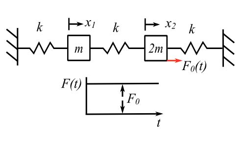
![\begin{equation*} [m] = \begin{bmatrix} m & 0 \\ 0 & 2m \\ \end{bmatrix} \end{equation*}](https://engcourses-uofa.ca/wp-content/ql-cache/quicklatex.com-e0ab99a2c898715f597ac02edf71cba7_l3.png "Rendered by QuickLaTeX.com")
![\begin{equation*} [k] = k \begin{bmatrix} 2 & -1 \\ -1 & 2 \\ \end{bmatrix} \end{equation*}](https://engcourses-uofa.ca/wp-content/ql-cache/quicklatex.com-ca6010155440f4742aa962c210ef03a9_l3.png "Rendered by QuickLaTeX.com")
Therefore

Characteristic equation is:
![\[(2k - mp^{2})(2k - 2mp^{2}) - k^{2} = 0\]](https://engcourses-uofa.ca/wp-content/ql-cache/quicklatex.com-883c01ac15e78681aef9379cba11f8fa_l3.png "Rendered by QuickLaTeX.com")
![\[4k^{2} - 6mp^{2}k+ 2m^{2}p^{4} - k^{2} = 0\]](https://engcourses-uofa.ca/wp-content/ql-cache/quicklatex.com-166071d45107ad0b57be7dfcf004cd69_l3.png "Rendered by QuickLaTeX.com")
![\[p^{4} - 3\frac{k}{m} p^{2} + \frac{3}{2} \bigg( \frac{k}{m} \bigg)^{2} = 0\]](https://engcourses-uofa.ca/wp-content/ql-cache/quicklatex.com-9c4c9c167f2adef43b8cae6f1fb31fb8_l3.png "Rendered by QuickLaTeX.com")
![\[\begin{split} p^2 &= \bigg[ \frac{3}{2} \pm \sqrt{\frac{9}{4} - \frac{3}{2}} \bigg] \frac{k}{m} \\&= \bigg( \frac{3}{2} \pm \frac{\sqrt{3}}{2} \bigg)\frac{k}{m} \end{split}\]](https://engcourses-uofa.ca/wp-content/ql-cache/quicklatex.com-dc2e032353a6d25cbc4402a87c1c9999_l3.png "Rendered by QuickLaTeX.com")
![\[\begin{split} p_{1}^{2} &= \bigg( \frac{3-\sqrt{3}}{2} \bigg) \frac{k}{m} \\&= 0.634 \frac{k}{m} \end{split}\]](https://engcourses-uofa.ca/wp-content/ql-cache/quicklatex.com-f02490386e676dbaa4458f12f0904119_l3.png "Rendered by QuickLaTeX.com")
![\[p_{1} = 0.796 \frac{k}{m}\]](https://engcourses-uofa.ca/wp-content/ql-cache/quicklatex.com-68306eadb34ad089da4841fb01ee94c6_l3.png "Rendered by QuickLaTeX.com")
![\[\begin{split} p_{2}^{2} &= \bigg( \frac{3+\sqrt{3}}{2} \bigg)\frac{k}{m} \\&= 2.366 \frac{k}{m} \end{split}\]](https://engcourses-uofa.ca/wp-content/ql-cache/quicklatex.com-76afc475d96524724a9d000114876b1f_l3.png "Rendered by QuickLaTeX.com")
![\[p_{2} = 1.5382 \sqrt{\frac{k}{m}}\]](https://engcourses-uofa.ca/wp-content/ql-cache/quicklatex.com-446e8cc0e9cbb3dab7b11e49b670a701_l3.png "Rendered by QuickLaTeX.com")
![\[\begin{split} \bigg( \frac{u_{2}}{u_{1}} \bigg)_{1} &= 2 - \frac{mp_{1}^{2}}{m} \\&= 2- 0.634 \\&= 1.366 \end{split}\]](https://engcourses-uofa.ca/wp-content/ql-cache/quicklatex.com-79b68b2ef9f6dbcd63b81d8229aef782_l3.png "Rendered by QuickLaTeX.com")
![\[\begin{split} \bigg( \frac{u_{2}}{u_{1}} \bigg)_{2} &= 2 - \frac{mp_{2}^{2}}{m} \\&= 2- 2.366 \\&= -0.366 \end{split}\]](https://engcourses-uofa.ca/wp-content/ql-cache/quicklatex.com-20ab4fdff0bbba5e2e55922fae413c41_l3.png "Rendered by QuickLaTeX.com")

![\[\{\mu\}_{1} = \alpha _{1} \{u\}_{1} \]](https://engcourses-uofa.ca/wp-content/ql-cache/quicklatex.com-6c80913985bd937fbb2d06d7e22a8776_l3.png "Rendered by QuickLaTeX.com")
Therefore,

Therefore,

Similarly:

now find the force vector in the normal coordinates
![\begin{equation*} \{N(t)\} = [u]^{T} \begin{Bmatrix} 0 \\ F_o \\ \end{Bmatrix} = \frac{1}{\sqrt{m}} \begin{bmatrix} 0.4597 & 0.6280\\ 0.8881 & -0.3251\\ \end{bmatrix} \begin{Bmatrix} 0 \\ F_o \\ \end{Bmatrix} = \frac{F_o}{\sqrt{m}} \begin{Bmatrix} 0.6280 \\ -0.3251 \\ \end{Bmatrix} \end{equation*}](https://engcourses-uofa.ca/wp-content/ql-cache/quicklatex.com-096501d47715852fe5694c94e1c692ec_l3.png "Rendered by QuickLaTeX.com")
Since there are initial conditions with no displacement and no velocity we can simply integrate the convolution integrals to give
![\[\begin{split} \eta_{1}(t) &= \frac{0.6280 F_{o}}{p_1 \sqrt{m}} \int_{0}^{t} \sin p(t-\tau ) \,d \tau \\&= \frac{0.6280 F_{o}}{p_{1}^{2} \sqrt{m}}(1- \cos p_{1} t) \end{split}\]](https://engcourses-uofa.ca/wp-content/ql-cache/quicklatex.com-ec2415f4a030160e0bf78d0e750fa0e4_l3.png "Rendered by QuickLaTeX.com")
![\[\eta_{2}(t) =\frac{-0.3251 F_{o}}{p_{2}^{2} \sqrt{m}}(1 - \cos p_{2} t)\]](https://engcourses-uofa.ca/wp-content/ql-cache/quicklatex.com-cc8fd4c0b851f6d4e70b838004060fe6_l3.png "Rendered by QuickLaTeX.com")
We can now find the response in terms of the original coordinates using:
![\[\{x(t)\} = \{\mu\}_{1} \eta _{1} (t) + \{\mu\}_{2} \eta _{2} (t)\]](https://engcourses-uofa.ca/wp-content/ql-cache/quicklatex.com-83ef1dcbb9e99a2e0f7a81792d4c3cd8_l3.png "Rendered by QuickLaTeX.com")
![\[\begin{split} x_{1}(t) &= \frac{(0.4597)(0.6280)F_{o}}{p_{1}^{2} m} \bigg(1 - \cos p_1 t \bigg) + \frac{(0.8881)(-0.3251)F_{o}}{p_{2}^{2} m} \bigg(1 - \cos p_2 t \bigg) \\&= \frac{F_o}{k} \frac{(0.4597)(0.6280)}{(0.634)} \bigg(1- \cos(0.796) \sqrt{\frac{k}{m}} t \bigg) + \frac{F_o}{k} \frac{(0.8881)(-0.3251)}{(2.366)} \bigg(1- \cos(1.5382) \sqrt{\frac{k}{m}} t \bigg) \end{split}\]](https://engcourses-uofa.ca/wp-content/ql-cache/quicklatex.com-fae9e285d8731592631f54a99ed0a96b_l3.png "Rendered by QuickLaTeX.com")
![\[x_{1}(t) = \frac{F_{o}}{k} \bigg[0.4553 \bigg(1- \cos 0.796 \sqrt{\frac{k}{m}}t \bigg) - 0.1220 \bigg(1 - \cos 1.5382 \sqrt{\frac{k}{m}}t \bigg) \bigg]\]](https://engcourses-uofa.ca/wp-content/ql-cache/quicklatex.com-d7eac8c52c792e067c0f67a2b1ad7c29_l3.png "Rendered by QuickLaTeX.com")
![\[x_{2}(t) = \frac{F_{o}}{k} \bigg[0.6219\bigg(1- \cos 0.796 \sqrt{\frac{k}{m}}t\bigg) +0.0447\bigg(1 - \cos 1.5382 \sqrt{\frac{k}{m}}t \bigg) \bigg]\]](https://engcourses-uofa.ca/wp-content/ql-cache/quicklatex.com-21e23e373cdaa2a7d6bcccc698066848_l3.png "Rendered by QuickLaTeX.com")
Note that the first mode is most pronounced in the overall response.
Check static deflection:
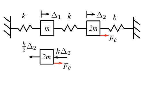
Therefore,  ,
, 
![\[\begin{split} x_2 \text{(static)} &= \frac{F_o}{k} (0.6219 + 0.0447) \\&= \Delta _2 \\&= \frac{F}{k} (0.6666) \qquad \text{O.K.} \end{split}\]](https://engcourses-uofa.ca/wp-content/ql-cache/quicklatex.com-c6d883562d1644538e48bb9586ee2ca8_l3.png "Rendered by QuickLaTeX.com")
![\[\begin{split} x_1 \text{(static)} &= \Delta _1 \\&= \frac{\Delta _2}{2} \\&= \frac{F_o}{k} (0.4553 - 0.1220) \\&= \frac{F_{o}}{3k} \\&= 0.3333\frac{F_{o}}{k} \qquad \text{O.K.} \end{split}\]](https://engcourses-uofa.ca/wp-content/ql-cache/quicklatex.com-30bf208e2aae8963771fdae516bed7a6_l3.png "Rendered by QuickLaTeX.com")
Consider a second example with certain initial conditions:
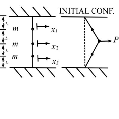
A static force  is suddenly released for the system of 3 masses mounted on a tightly stretched wire with tension
  . Determine the resulting free vibration using normal mode analysis.
Solution:
While the mass matrix is easy we must find the stiffness matrix using say 
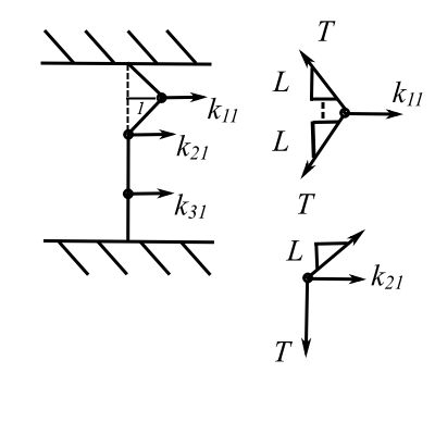
Apply unit deflection to  ,
,
![\[\begin{split} \sum F_{x} &= 0 \\&= k_{11} - T \left(\frac{1}{L}\right) - T \left(\frac{1}{L}\right) \end{split}\]](https://engcourses-uofa.ca/wp-content/ql-cache/quicklatex.com-eb6a3b78c23a52503441fcecb8184cb5_l3.png "Rendered by QuickLaTeX.com")
Therefore,
![\[k_{11} = \frac{2T}{L}\]](https://engcourses-uofa.ca/wp-content/ql-cache/quicklatex.com-e50cc357fd09a8035b3c95e5cfa4ff7f_l3.png "Rendered by QuickLaTeX.com")
![\[k_{21} = \frac{-T}{L}\]](https://engcourses-uofa.ca/wp-content/ql-cache/quicklatex.com-86399399e4c0308b5e0e5ca9825d104f_l3.png "Rendered by QuickLaTeX.com")
![\[k_{31} = 0\]](https://engcourses-uofa.ca/wp-content/ql-cache/quicklatex.com-394f89ebcc16ecf9944381f21d78eedf_l3.png "Rendered by QuickLaTeX.com")
Therefore,

now find the ‘s &  , assume
  to get:

where
![\[ \lambda = \frac{p^{2}mL}{T}\]](https://engcourses-uofa.ca/wp-content/ql-cache/quicklatex.com-f39b8da9764a2118a849c930c08b9bda_l3.png "Rendered by QuickLaTeX.com")
The characteristic equation is 
![\[(2-\lambda)[(2-\lambda)^{2} - 2] = (2-\lambda)[\lambda ^{2} -4 \lambda + 2] = 0\]](https://engcourses-uofa.ca/wp-content/ql-cache/quicklatex.com-9f43e3febe23ec02df0d5779c64be9ca_l3.png "Rendered by QuickLaTeX.com")
 or
or 
Therefore,
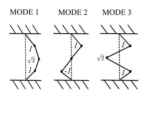
![\[\lambda _1 = 2- \sqrt{2}, \lambda _2 = 2, \lambda _3 = 2+ \sqrt{2}\]](https://engcourses-uofa.ca/wp-content/ql-cache/quicklatex.com-b2c542e2807de6796d42ab435705e26e_l3.png "Rendered by QuickLaTeX.com")
![\[p_{1}^{2} = (2- \sqrt{2}) \frac{T}{mL}, p_{2}^{2} = 2 \frac{T}{mL}, p_{3}^{2} = (2+ \sqrt{2})\frac{T}{mL}\]](https://engcourses-uofa.ca/wp-content/ql-cache/quicklatex.com-1aaf71ee5f3ceb38f76c071eafee66c6_l3.png "Rendered by QuickLaTeX.com")
now find  , choose
![\[(2- \lambda) - u_{2} = 0\]](https://engcourses-uofa.ca/wp-content/ql-cache/quicklatex.com-d93d071347b03416903dfb4f1630c6a0_l3.png "Rendered by QuickLaTeX.com")
![\[-1 + (2- \lambda)u_{2} - u_{3} = 0\]](https://engcourses-uofa.ca/wp-content/ql-cache/quicklatex.com-64a664fecd40b6bdad8d089b13313d32_l3.png "Rendered by QuickLaTeX.com")
![\[-u_{2} + (2- \lambda)u_{3} = 0\]](https://engcourses-uofa.ca/wp-content/ql-cache/quicklatex.com-7722b866b68161c7da4c188368ba6987_l3.png "Rendered by QuickLaTeX.com")
For 
For 
For 
Therefore,


now normalize the  to get
  where
where  , therefore as
 ![\{\mu\}^{T} [m] \{\mu\} = 1](https://engcourses-uofa.ca/wp-content/ql-cache/quicklatex.com-d70bba31e19ca1e7a045d18d2c6a2878_l3.png "Rendered by QuickLaTeX.com")

![\[\alpha_1 = \frac{1}{2\sqrt{m}}\]](https://engcourses-uofa.ca/wp-content/ql-cache/quicklatex.com-42b3294ad797d73d53153298c9f2757d_l3.png "Rendered by QuickLaTeX.com")

Similarly,


Therefore,

Also need the initial conditions
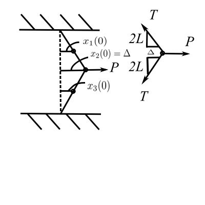
Therefore
![\[P = 2 \frac{\Delta}{2L} T\]](https://engcourses-uofa.ca/wp-content/ql-cache/quicklatex.com-1afd136a83b33b6a064a1609f208a06a_l3.png "Rendered by QuickLaTeX.com")
![\[x_{2}(0) = \Delta = \frac{PL}{T}\]](https://engcourses-uofa.ca/wp-content/ql-cache/quicklatex.com-b379bc0cc4926008c42fb572f7935297_l3.png "Rendered by QuickLaTeX.com")
![\[x_{1}(0) = x_{3}(0) = \frac{\Delta}{2} = \frac{PL}{2T}\]](https://engcourses-uofa.ca/wp-content/ql-cache/quicklatex.com-1f8cef74681f8ead8c4d684ddeccaa1d_l3.png "Rendered by QuickLaTeX.com")
![\[\dot{x}_{1,2,3}(0) = 0\]](https://engcourses-uofa.ca/wp-content/ql-cache/quicklatex.com-2726e515a4e1797f0ece9540a29f64ff_l3.png "Rendered by QuickLaTeX.com")

![\[\{\dot{x}(0)\} = \{0\}\]](https://engcourses-uofa.ca/wp-content/ql-cache/quicklatex.com-edce4c5696c47d421d0467e03d800b66_l3.png "Rendered by QuickLaTeX.com")
We can simply put this into the general solution:
![\[\{x(t)\} =\sum_{r=1}^{3} [\{\mu\}_{r}^{T} [m] \{x(0)\} \cos p_{r}(t) + \{\mu\}_{r}^{T}[m] \{\dot{x}(0)\}\frac{1}{p_{r}} \sin p_{r}(t)] \{\mu\}_{r}\]](https://engcourses-uofa.ca/wp-content/ql-cache/quicklatex.com-d237297b563a744315313471ca5e77c8_l3.png "Rendered by QuickLaTeX.com")


![\[x_{1}(t) = (2+2\sqrt{2})\frac{PL}{8T} \cos p_{1}(t) + (2-2\sqrt{2})\frac{PL}{8T} \cos p_{3}(t)\]](https://engcourses-uofa.ca/wp-content/ql-cache/quicklatex.com-4dbcdf2e4c40875f06eed5b7ddaf725c_l3.png "Rendered by QuickLaTeX.com")
![\[x_{2}(t) = (4+2\sqrt{2})\frac{PL}{8T} \cos p_{1}(t) + (4-2\sqrt{2})\frac{PL}{8T} \cos p_{3}(t)\]](https://engcourses-uofa.ca/wp-content/ql-cache/quicklatex.com-1dabacaf650bc966ae14f2bd2befeed3_l3.png "Rendered by QuickLaTeX.com")
![\[x_{3}(t) = (2+2\sqrt{2})\frac{PL}{8T} \cos p_{1}(t) + (2-2\sqrt{2})\frac{PL}{8T} \cos p_{3}(t)\]](https://engcourses-uofa.ca/wp-content/ql-cache/quicklatex.com-46cc3d9160b235ec302985a839d74729_l3.png "Rendered by QuickLaTeX.com")
Again the first mode is the dominant one and the second unsymmetric mode is not present. If we had chosen different initial condition, then
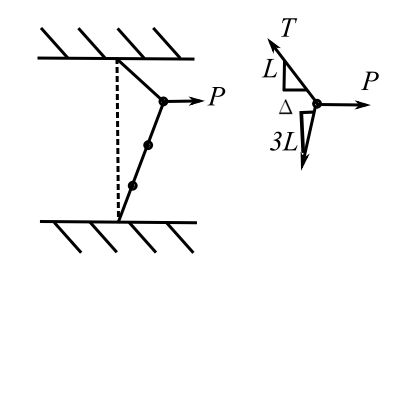
![\[\begin{split} p &= \frac{\Delta}{L}T + \frac{\Delta}{3L} T \\&= \frac{4}{3} \frac{\Delta T}{L} \end{split}\]](https://engcourses-uofa.ca/wp-content/ql-cache/quicklatex.com-560aa211ddf662ab8fbae37033420df1_l3.png "Rendered by QuickLaTeX.com")
![\[\begin{split} \Delta &= \frac{3}{4} \frac{PL}{T} \\&= x_{1}(0) \end{split}\]](https://engcourses-uofa.ca/wp-content/ql-cache/quicklatex.com-8260aab6ad33f422e67bc538ee2bef55_l3.png "Rendered by QuickLaTeX.com")
![\[\begin{split} x_{2}(0) &= \left(\frac{2}{3}\right) \left(\frac{3}{4}\right) \frac{PL}{T} \\&= \frac{PL}{2T} \end{split}\]](https://engcourses-uofa.ca/wp-content/ql-cache/quicklatex.com-0ca335c84653a1b80fe36b1ce590c995_l3.png "Rendered by QuickLaTeX.com")
![\[x_{1}(0) = \frac{PL}{4T}\]](https://engcourses-uofa.ca/wp-content/ql-cache/quicklatex.com-89048a91b80b6d436802b5a77108a227_l3.png "Rendered by QuickLaTeX.com")
Therefore

All three modes would now participate in the motion. To find the response simply insert the new and calculate the  .
.
e.g Steady State
The equations of motion are

Therefore,

![\[(3k-2mp^{2})(k-mp^{2})^{2}- k^{2}(k-mp^{2}) - k^{2}(k-mp^{2}) = 0\]](https://engcourses-uofa.ca/wp-content/ql-cache/quicklatex.com-ade25b77f3bbf484b452b68b4521f118_l3.png "Rendered by QuickLaTeX.com")
Divide by  and set
![\[(3-2\lambda)(1-\lambda)^{2}- (1-\lambda) - (1-\lambda) = 0\]](https://engcourses-uofa.ca/wp-content/ql-cache/quicklatex.com-bd5c884a121a5ecbd8e9f0ad0e5a4621_l3.png "Rendered by QuickLaTeX.com")
![\[(1-\lambda)[(3 - 2\lambda)(1 -\lambda) -2] = 0\]](https://engcourses-uofa.ca/wp-content/ql-cache/quicklatex.com-1524af2bcd4595df33f071a13c1c996f_l3.png "Rendered by QuickLaTeX.com")
Therefore,
![\[(1-\lambda)[3 - 5\lambda + 2\lambda ^{2} -2] = 0\]](https://engcourses-uofa.ca/wp-content/ql-cache/quicklatex.com-68315e766047e05450c6337c7f109983_l3.png "Rendered by QuickLaTeX.com")
![\[ \lambda = 1, \lambda = \frac{5 \pm \sqrt{25-8}}{4} = \frac{5 \pm \sqrt{17}}{4} \]](https://engcourses-uofa.ca/wp-content/ql-cache/quicklatex.com-481c07959638cbdccc0423f26159c75d_l3.png "Rendered by QuickLaTeX.com")
![\[\lambda = 0.21922, 1, 2.2808\]](https://engcourses-uofa.ca/wp-content/ql-cache/quicklatex.com-8f4fa21cbea1cff2c19f993108706de0_l3.png "Rendered by QuickLaTeX.com")
Note:  ,
,
![\[(3-2\lambda) A_{1} - A_{2} - A_{3} = 0 ---- \textcircled{1}\]](https://engcourses-uofa.ca/wp-content/ql-cache/quicklatex.com-91b2ecc0b57cc4b17795fcd7e268a841_l3.png "Rendered by QuickLaTeX.com")
![\[-A_{1} + (1-\lambda)A_{2} = 0 --- \textcircled{2}\]](https://engcourses-uofa.ca/wp-content/ql-cache/quicklatex.com-e1bda885aa8d956c01fa166db04b1ff7_l3.png "Rendered by QuickLaTeX.com")
![\[-A_{1} + (1-\lambda)A_{3} = 0 --- \textcircled{3}\]](https://engcourses-uofa.ca/wp-content/ql-cache/quicklatex.com-b645d849da8fbbcd31687658a0efdc04_l3.png "Rendered by QuickLaTeX.com")
For 
Therefore, from  and
and 
![\[A_{2} = A_{3} = 1\]](https://engcourses-uofa.ca/wp-content/ql-cache/quicklatex.com-88de92964eed00e60dc1ae6f30262df9_l3.png "Rendered by QuickLaTeX.com")
From  ,
,
![\[\bigg[3 - \frac{(5 - \sqrt{17})}{2}\bigg] A_{1} = 2\]](https://engcourses-uofa.ca/wp-content/ql-cache/quicklatex.com-b065f10445122140d3fc5b22735eafbb_l3.png "Rendered by QuickLaTeX.com")
![\[\begin{split} A_{1} &= \frac{2}{3 - \frac{5-\sqrt{17}}{2}} \\&= 0.78078 \end{split}\]](https://engcourses-uofa.ca/wp-content/ql-cache/quicklatex.com-75f84c11aca7aa560f5c76256bdafa78_l3.png "Rendered by QuickLaTeX.com")
Therefore:
![\[\begin{Bmatrix}A\end{Bmatrix}^1 =\begin{pmatrix}0.78078 \\ 1 \\ 1\end{pmatrix} \]](https://engcourses-uofa.ca/wp-content/ql-cache/quicklatex.com-3e95945ba328166380f8a4049bea9e8f_l3.png "Rendered by QuickLaTeX.com")
For 
 therefore
![\[\begin{Bmatrix}A\end{Bmatrix}^2 =\begin{pmatrix}0 \\ 1 \\ -1\end{pmatrix}\]](https://engcourses-uofa.ca/wp-content/ql-cache/quicklatex.com-023c3afa60c45a47e121d669c458a8b9_l3.png "Rendered by QuickLaTeX.com")
For 
Again 
![\[ \begin{split}A_1 &= \left(1 - \frac{5+\sqrt{17}}{4}\right)A_2 \\A_1 &= -1.28078\end{split}\]](https://engcourses-uofa.ca/wp-content/ql-cache/quicklatex.com-9510e1a5ade6853f27ced1be399cbc4c_l3.png "Rendered by QuickLaTeX.com")
Therefore:
![\[\begin{Bmatrix}A\end{Bmatrix}^3 =\begin{Bmatrix}-1.28078 \\ 1 \\ 1\end{Bmatrix}\]](https://engcourses-uofa.ca/wp-content/ql-cache/quicklatex.com-b36f6712154aef57d3bcece2cff86cba_l3.png "Rendered by QuickLaTeX.com")
Normalized eigenvectors
![\[ \begin{split} \alpha_1^2\begin{Bmatrix}A\end{Bmatrix}^T_1\begin{bmatrix}m\end{bmatrix}\begin{Bmatrix}A\end{Bmatrix}_1&= 1 \\ \alpha_1 &= \frac{0.55734}{\sqrt{m}} \\ \alpha_2^2\begin{Bmatrix}A\end{Bmatrix}^T_2\begin{bmatrix}m\end{bmatrix}\begin{Bmatrix}A\end{Bmatrix}_2&= 1 \\ \alpha_2 &= \frac{1}{\sqrt{2m}} = \frac{0.70711}{\sqrt{m}} \\ \alpha_3^2\begin{Bmatrix}A\end{Bmatrix}^T_3\begin{bmatrix}m\end{bmatrix}\begin{Bmatrix}A\end{Bmatrix}_3&= 1 \\ \alpha_3 &= \frac{0.43516}{\sqrt{m}} \end{split} \]](https://engcourses-uofa.ca/wp-content/ql-cache/quicklatex.com-a9e753116afbcc949c0e533bba054aa9_l3.png "Rendered by QuickLaTeX.com")
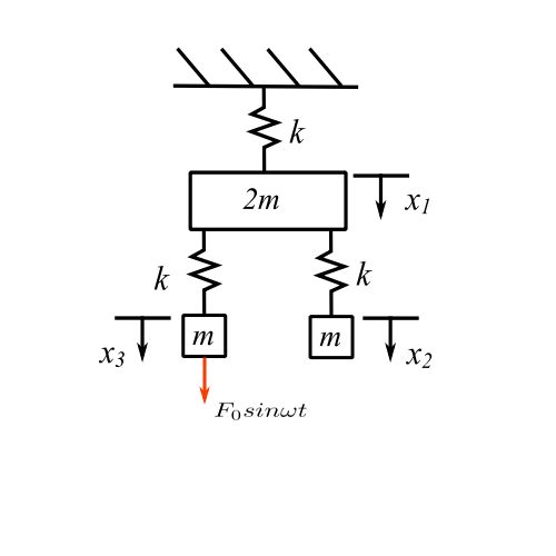
therefore:
![\[\begin{bmatrix}u\end{bmatrix} = \frac{1}{\sqrt{m}}\begin{bmatrix}0.43516 && 0 && -0.55734 \\0.55734 && 0.70711 && 0.43516 \\0.55734 && -0.70711 && 0.43516\end{bmatrix}\]](https://engcourses-uofa.ca/wp-content/ql-cache/quicklatex.com-681702ad6b95f13f9fcb48f81b4e9337_l3.png "Rendered by QuickLaTeX.com")
The transformed forces are:
![\[\begin{bmatrix}u\end{bmatrix}^T\begin{Bmatrix}0 \\ 0 \\ F_0\end{Bmatrix} \sin\omega t= \frac{F_0}{\sqrt{m}}\begin{Bmatrix}0.55734 \\ -0.70711 \\ 0.43516\end{Bmatrix}\sin \omega t\]](https://engcourses-uofa.ca/wp-content/ql-cache/quicklatex.com-bd631c62bc852bc2b1e6a320b27d6c31_l3.png "Rendered by QuickLaTeX.com")
Therefore transformed equations are:
![\[\begin{Bmatrix}\Ddot{\eta}\end{Bmatrix} +\begin{bmatrix}p^2\end{bmatrix}\eta =\frac{F_0}{\sqrt{m}}\begin{Bmatrix}0.55734 \\ -0.70711 \\ 0.43516\end{Bmatrix} \sin\omega t\]](https://engcourses-uofa.ca/wp-content/ql-cache/quicklatex.com-b9bb9be93915c6c9d772fab43e50a47d_l3.png "Rendered by QuickLaTeX.com")
Steady State Solutions of these equations
![\[\eta_1 = \frac{0.55734\frac{F_0}{\sqrt{m}}}{(p_1-\omega^2)} \sin\omega t \]](https://engcourses-uofa.ca/wp-content/ql-cache/quicklatex.com-f3ec1505c55091fafadeca4e9ec3faea_l3.png "Rendered by QuickLaTeX.com")
![\[\eta_2 = \frac{-0.70711\frac{F_0}{\sqrt{m}}}{(p_2^2-\omega^2)} \sin\omega t \]](https://engcourses-uofa.ca/wp-content/ql-cache/quicklatex.com-eb5bf049e683b278c6dea4f42d992904_l3.png "Rendered by QuickLaTeX.com")
![\[\eta_3 = \frac{0.43516\frac{F_0}{\sqrt{m}}}{(p_3^2-\omega^2)} \sin\omega t\]](https://engcourses-uofa.ca/wp-content/ql-cache/quicklatex.com-708dcde4714cfba20c60ca7a0e2aec2a_l3.png "Rendered by QuickLaTeX.com")
![\[ \begin{split}\begin{Bmatrix}x\end{Bmatrix} &= \begin{bmatrix}u\end{bmatrix}\begin{Bmatrix}\eta\end{Bmatrix} \\&= \frac{F_0}{k}\begin{bmatrix}0.43516 && 0 && -0.55734 \\0.55734 && 0.70711 && 0.43516 \\0.55734 && -0.70711 && 0.43516\end{bmatrix}\begin{Bmatrix}\frac{0.55734}{(1-\frac{\omega^2}{P_1^2})} \\\frac{-0.70711}{(1-\frac{\omega^2}{P_2^2})} \\\frac{0.43516}{(1-\frac{\omega^2}{P_3^2})}\end{Bmatrix}\sin\omega t\end{split} \]](https://engcourses-uofa.ca/wp-content/ql-cache/quicklatex.com-d18ef44b8249038f38ceee5a8493edc0_l3.png "Rendered by QuickLaTeX.com")
For the case in which we have repeated eigenvalues we can still have orthogonal eigenvectors using a process called successive orthogonalization.
If the eigenvalues is repeated  times let
  be an arbitrary set of modal vectors that satisfy the degenerate set of equations. We construct an orthoganal set using
![\[ \begin{Bmatrix}u\end{Bmatrix}_1 = \begin{Bmatrix}u\end{Bmatrix}_{p_1} \]](https://engcourses-uofa.ca/wp-content/ql-cache/quicklatex.com-cbd0a86648ccd451ce691e1a7a9f9fee_l3.png "Rendered by QuickLaTeX.com")
![\[ \begin{Bmatrix}u\end{Bmatrix}_2 = \begin{Bmatrix}u\end{Bmatrix}_{p_2} - \frac{\begin{Bmatrix}u\end{Bmatrix}^T_1 \begin{bmatrix}m\end{bmatrix} \begin{Bmatrix}u\end{Bmatrix}_{p_2}}{\begin{Bmatrix}u\end{Bmatrix}^T_1 \begin{bmatrix}m\end{bmatrix} \begin{Bmatrix}u\end{Bmatrix}_1} \]](https://engcourses-uofa.ca/wp-content/ql-cache/quicklatex.com-4c0f025ecae4e2ad28143ae8155f6b4f_l3.png "Rendered by QuickLaTeX.com")
![\[ \begin{Bmatrix}u\end{Bmatrix}_3 = \begin{Bmatrix}u\end{Bmatrix}_{p_3} - \frac{\begin{Bmatrix}u\end{Bmatrix}^T_2 \begin{bmatrix}m\end{bmatrix} \begin{Bmatrix}u\end{Bmatrix}_{p_3}}{\begin{Bmatrix}u\end{Bmatrix}^T_2 \begin{bmatrix}m\end{bmatrix} \begin{Bmatrix}u\end{Bmatrix}_2} \begin{Bmatrix}u\end{Bmatrix}_2 - \frac{\begin{Bmatrix}u\end{Bmatrix}^T_1 \begin{bmatrix}m\end{bmatrix} \begin{Bmatrix}u\end{Bmatrix}_{p_3}}{\begin{Bmatrix}u\end{Bmatrix}^T_1 \begin{bmatrix}m\end{bmatrix} \begin{Bmatrix}u\end{Bmatrix}_1} \begin{Bmatrix}u\end{Bmatrix}_1 \]](https://engcourses-uofa.ca/wp-content/ql-cache/quicklatex.com-5ef7f2e8ef3663d37d3a36b06b8b2c80_l3.png "Rendered by QuickLaTeX.com")
etc.
To prove take
![\[\begin{Bmatrix}u\end{Bmatrix}^T_1 \begin{bmatrix}m\end{bmatrix} \begin{Bmatrix}u\end{Bmatrix}_2 = \begin{Bmatrix}u\end{Bmatrix}^T_1 \begin{bmatrix}m\end{bmatrix} \begin{Bmatrix}u\end{Bmatrix}_{p_2} -\frac{\begin{Bmatrix}u\end{Bmatrix}^T_1 \begin{bmatrix}m\end{bmatrix} \begin{Bmatrix}u\end{Bmatrix}_{p_2}}{\begin{Bmatrix}u\end{Bmatrix}^T_1 \begin{bmatrix}m\end{bmatrix} \begin{Bmatrix}u\end{Bmatrix}_1} \begin{Bmatrix}u\end{Bmatrix}^T_1 \begin{bmatrix}m\end{bmatrix} \begin{Bmatrix}u\end{Bmatrix}_1 = \underline{\underline{0}}\]](https://engcourses-uofa.ca/wp-content/ql-cache/quicklatex.com-f898af77b0b9b27fa25f5351bd244c99_l3.png "Rendered by QuickLaTeX.com")
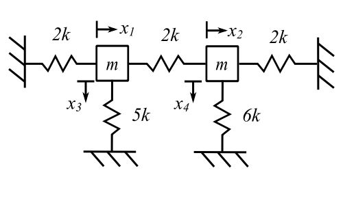
![\[ \begin{bmatrix}m\end{bmatrix} = m \begin{bmatrix}1 && 0 && 0 && 0 \\0 && 1 && 0 && 0 \\0 && 0 && 1 && 0 \\0 && 0 && 0 && 1\end{bmatrix}\]](https://engcourses-uofa.ca/wp-content/ql-cache/quicklatex.com-4a7e3274d4c10acecf2846318ea0862e_l3.png "Rendered by QuickLaTeX.com")
![\[ \begin{bmatrix}k\end{bmatrix} = k \begin{bmatrix}4 && -2 && 0 && 0 \\-2 && 4 && 0 && 0 \\0 && 0 && 5 && 0 \\0 && 0 && 0 && 6\end{bmatrix}\]](https://engcourses-uofa.ca/wp-content/ql-cache/quicklatex.com-8058b51477c21fc95c44cc8f638acc23_l3.png "Rendered by QuickLaTeX.com")
The characteristic equation is
![\[ \begin{Bmatrix}\begin{bmatrix}k\end{bmatrix} -p^2\begin{bmatrix}m\end{bmatrix}\end{Bmatrix}\begin{Bmatrix}u\end{Bmatrix} = 0\]](https://engcourses-uofa.ca/wp-content/ql-cache/quicklatex.com-c3be4fc244f321a2122b5bf904660c88_l3.png "Rendered by QuickLaTeX.com")
![\[ \lambda \equiv \frac{p^2m}{k} \]](https://engcourses-uofa.ca/wp-content/ql-cache/quicklatex.com-f77b1b0557667c65b8a57f9816291a72_l3.png "Rendered by QuickLaTeX.com")
Therefore
![\[ \begin{vmatrix}4-\lambda && -2 && 0 && 0 \\-2 && 4-\lambda && 0 && 0 \\0 && 0 && 5-\lambda && 0 \\0 && 0 && 0 && 6-\lambda\end{vmatrix} = 0 \]](https://engcourses-uofa.ca/wp-content/ql-cache/quicklatex.com-7af809d3ec8740523d30a3190593c905_l3.png "Rendered by QuickLaTeX.com")
![\[ \begin{split}&= (6-\lambda)\biggr[(4-\lambda)^2(5-\lambda)-4(5-\lambda)\biggr] \\&= (6-\lambda)(5-\lambda)(12-8\lambda+\lambda^2) \\&= (6-\lambda)(5-\lambda)(6-\lambda)(2-\lambda)\end{split} \]](https://engcourses-uofa.ca/wp-content/ql-cache/quicklatex.com-cfbe6529faaa398dc4748c398dfb6adf_l3.png "Rendered by QuickLaTeX.com")
Therefore: 
For the repeated root 
![\[ \begin{split}-2u_1-2u_2 &=0 \\-2u_1-2u_2 &= 0 \\u_3 &= 0 \\u_4 &= ?\end{split} \]](https://engcourses-uofa.ca/wp-content/ql-cache/quicklatex.com-b7395aa546c9b1e9faf4aef1adb5ed27_l3.png "Rendered by QuickLaTeX.com")
from
![\[ \begin{bmatrix}4-\lambda && -2 && 0 && 0 \\-2 && 4-\lambda && 0 && 0 \\0 && 0 && 5-\lambda && 0 \\0 && 0 && 0 && 6-\lambda\end{bmatrix} \begin{Bmatrix}u_1 \\ u_2 \\ u_3 \\ u_4\end{Bmatrix} = \begin{Bmatrix}0 \\ 0 \\ 0 \\ 0\end{Bmatrix}\]](https://engcourses-uofa.ca/wp-content/ql-cache/quicklatex.com-d8a5a54f06c64edccc4cfbb7b61b3f1e_l3.png "Rendered by QuickLaTeX.com")
Therefore there are an infinite number of solutions so choose one which satisfies the equations. e.g.:
![\[ \begin{Bmatrix}u\end{Bmatrix}_1^{\ast} =\begin{bmatrix} 1 \\ -1 \\ 0 \\ 2 \end{bmatrix} =\begin{Bmatrix}u\end{Bmatrix}_1 \]](https://engcourses-uofa.ca/wp-content/ql-cache/quicklatex.com-cd10cd4ddca18e9a32ed9db591864677_l3.png "Rendered by QuickLaTeX.com")
![\[ \begin{Bmatrix}u\end{Bmatrix}_2^{\ast} =\begin{Bmatrix} 2 \\ -2 \\ 0 \\ 0\end{Bmatrix} \]](https://engcourses-uofa.ca/wp-content/ql-cache/quicklatex.com-7f1f6bc2688dfb709fb4bae555a18956_l3.png "Rendered by QuickLaTeX.com")
Now we make them orthogonal
![\[ \begin{split}\begin{Bmatrix}u\end{Bmatrix}_2 &= \begin{Bmatrix}u\end{Bmatrix}_2^{\ast} -\frac{\begin{Bmatrix}u\end{Bmatrix}^T_1 \begin{bmatrix}m\end{bmatrix} \begin{Bmatrix}u\end{Bmatrix}_2^{\ast}}{\begin{Bmatrix}u\end{Bmatrix}^T_1 \begin{bmatrix}m\end{bmatrix} \begin{Bmatrix}u\end{Bmatrix}_1} \begin{Bmatrix}u\end{Bmatrix}_1 \\&= \begin{Bmatrix}2 \\ -2 \\ 0 \\ 0\end{Bmatrix}-\frac{1}{6}\begin{bmatrix}1 && -1 && 0 && 2\end{bmatrix}\begin{bmatrix}2 \\ -2 \\ 0 \\ 0\end{bmatrix}\begin{Bmatrix}u\end{Bmatrix}_1 \\&= \frac{4}{3}\begin{Bmatrix}1 \\ -1 \\ 0 \\ -1\end{Bmatrix}\end{split}\]](https://engcourses-uofa.ca/wp-content/ql-cache/quicklatex.com-bdbae36d03e17dc0e179e2416b978af1_l3.png "Rendered by QuickLaTeX.com")
Now  and
and  are orthonormal. For
  therefore:
![\[ \begin{Bmatrix}u\end{Bmatrix}_3 = \begin{bmatrix}1 \\ 1 \\ 0 \\ 0\end{bmatrix} \]](https://engcourses-uofa.ca/wp-content/ql-cache/quicklatex.com-530a129b5a9eff18d277da71d999f3f6_l3.png "Rendered by QuickLaTeX.com")
For 
![\[\begin{Bmatrix}u\end{Bmatrix}_4=\begin{bmatrix} 0 \\ 0 \\ 1 \\ 0\end{bmatrix} \]](https://engcourses-uofa.ca/wp-content/ql-cache/quicklatex.com-9b897268166a4c9483b401e8a6955ff2_l3.png "Rendered by QuickLaTeX.com")
and this is our basis.
Proportional Damping
Now consider the addition of damping to the system
![\[ \begin{bmatrix}m\end{bmatrix}\begin{Bmatrix}\Ddot{x}\end{Bmatrix} +\begin{bmatrix}c\end{bmatrix}\begin{Bmatrix}\dot{x}\end{Bmatrix} +\begin{bmatrix}k\end{bmatrix}\begin{Bmatrix}x\end{Bmatrix} =\begin{Bmatrix}F(t)\end{Bmatrix} \]](https://engcourses-uofa.ca/wp-content/ql-cache/quicklatex.com-d8063a9192c69d3b651abfed129bc328_l3.png "Rendered by QuickLaTeX.com")
Now transform this to normal coordinates
![\[ \begin{Bmatrix}x\end{Bmatrix} = \begin{bmatrix} \mu \end{bmatrix} \begin{Bmatrix}\eta(t) \end{Bmatrix} \]](https://engcourses-uofa.ca/wp-content/ql-cache/quicklatex.com-de5d1ad5a0b2ac5157d993aed3df4338_l3.png "Rendered by QuickLaTeX.com")
and premultiply by 
![\[\begin{bmatrix}\mu\end{bmatrix}^T\begin{bmatrix}m\end{bmatrix}\begin{bmatrix}\mu\end{bmatrix}\begin{Bmatrix}\Ddot{\eta}(t)\end{Bmatrix} +\begin{bmatrix}\mu\end{bmatrix}^T\begin{bmatrix}c\end{bmatrix}\begin{bmatrix}\mu\end{bmatrix}\begin{Bmatrix}\dot{\eta}(t)\end{Bmatrix} +\begin{bmatrix}\mu\end{bmatrix}^T\begin{bmatrix}k\end{bmatrix}\begin{bmatrix}\mu\end{bmatrix}\begin{Bmatrix}\eta(t)\end{Bmatrix} =\begin{bmatrix}\mu\end{bmatrix}^T\begin{Bmatrix}F(t)\end{Bmatrix}\]](https://engcourses-uofa.ca/wp-content/ql-cache/quicklatex.com-c561990829b107e67f2957caf89c9a99_l3.png "Rendered by QuickLaTeX.com")
therefore:
![\[\begin{Bmatrix}\Ddot{\eta}(t)\end{Bmatrix} +\begin{bmatrix}\mu\end{bmatrix}^T\begin{bmatrix}c\end{bmatrix}\begin{bmatrix}\mu\end{bmatrix}\begin{Bmatrix}\dot{\eta}(t)\end{Bmatrix} +\begin{bmatrix}p^2\end{bmatrix}\begin{Bmatrix}\eta(t)\end{Bmatrix} =\begin{Bmatrix}N(t)\end{Bmatrix}\]](https://engcourses-uofa.ca/wp-content/ql-cache/quicklatex.com-78afc8b626656070d3598ec4f0f8e3d4_l3.png "Rendered by QuickLaTeX.com")
but there is no a priori reason that  is a diagonal matrix and therefore the equations are coupled. If it was, we could use the same approach as before. One condition that is often used is the so-called proportional damping where
![\[\begin{bmatrix}c\end{bmatrix} = \alpha \begin{bmatrix}m\end{bmatrix} + \beta \begin{bmatrix}k\end{bmatrix}\]](https://engcourses-uofa.ca/wp-content/ql-cache/quicklatex.com-9ddfc90d1abd6a9021c37ba1f27c09d3_l3.png "Rendered by QuickLaTeX.com")
so that the transformed equations are necessarily diagonal. We can then set
![\[\begin{bmatrix}\mu\end{bmatrix}^T\begin{bmatrix}c\end{bmatrix}\begin{bmatrix}\mu\end{bmatrix} :=\begin{bmatrix}2\nu p\end{bmatrix}\]](https://engcourses-uofa.ca/wp-content/ql-cache/quicklatex.com-3742d07ace7f61c930b9c38f789612bc_l3.png "Rendered by QuickLaTeX.com")
then each transformed equation is
![\[ \Ddot\eta_r(t) + 2\nu_rp_r\dot\eta_r(t) + p_r^2\eta(t) = N_r(t) \]](https://engcourses-uofa.ca/wp-content/ql-cache/quicklatex.com-93646d073712a679df0f96a0e21a17a2_l3.png "Rendered by QuickLaTeX.com")
The general solution of this equation is
![\[ \begin{split}\eta_r(t) &= \frac{1}{\sqrt{1-\nu^2_r}p_r} \int_0^tN_r(t)e^{-\nu_r p_r(t-\tau)} \sin{\sqrt{1-\nu_r^2}} p_r(t-\tau)d\tau \\ &+ e^{-\nu_r p_r t} \biggr[\frac{\eta_r(0)}{\sqrt{1-\nu^2_r}}\cos(\sqrt{1-\nu_r^2}p_rt-\Psi_r) + \frac{\dot\eta(0)}{\sqrt{1-\nu^2_r}p_r} \sin\sqrt{1-\nu_r^2}p_r t \biggr]\end{split}\]](https://engcourses-uofa.ca/wp-content/ql-cache/quicklatex.com-81ca36755361084b9768be90cb267e89_l3.png "Rendered by QuickLaTeX.com")
where 
Now consider that the  are related
![\[ \begin{split}\begin{bmatrix}\mu\end{bmatrix}^T\begin{bmatrix}c\end{bmatrix}\begin{bmatrix}\mu\end{bmatrix} &=\alpha \begin{bmatrix}\mu\end{bmatrix}^T\begin{bmatrix}m\end{bmatrix}\begin{bmatrix}\mu\end{bmatrix} +\beta \begin{bmatrix}\mu\end{bmatrix}^T\begin{bmatrix}k\end{bmatrix}\begin{bmatrix}\mu\end{bmatrix} \\&= \alpha \begin{bmatrix}I\end{bmatrix} +\beta \begin{bmatrix}p^2\end{bmatrix} \\ &:=\begin{bmatrix} 2\nu p \end{bmatrix}\end{split}\]](https://engcourses-uofa.ca/wp-content/ql-cache/quicklatex.com-97abaa9c8a1d21020c524452af93fe47_l3.png "Rendered by QuickLaTeX.com")
therefore
![\[ \begin{split}\alpha +\beta p_i^2 &= 2\nu_i p_i \\\nu_i &= \frac{1}{2p_i}(\alpha+\beta p_i^2) \\ &=\frac{\alpha}{2p_i} + \frac{\beta p_i}{2}\end{split} \]](https://engcourses-uofa.ca/wp-content/ql-cache/quicklatex.com-fd0fcc188dae1a443669f8859cb6e872_l3.png "Rendered by QuickLaTeX.com")
Therefore we can only choose the damping independently for 2 modes. If  then
then  so that the damping in each mode is proportional to the frequency of that mode. The higher the frequency the higher the damping so that higher modes damp out more rapidly. [Note: Often called relative damping.]
On the other hand, setting  implies the damping is proportional to the mass matrix
  which damps out the lower modes more than the higher ones. [Note: Often called absolute damping.]
Return to a simple problem we have done previously

![\[ \begin{bmatrix}m && 0 \\ 0 && m\end{bmatrix} \begin{Bmatrix}\Ddot{x}_1 \\ \Ddot{x}_2\end{Bmatrix} + \begin{bmatrix}k+k_c && -k_c \\ -k_c && k+k_c\end{bmatrix} \begin{Bmatrix}x_1 \\ x_2\end{Bmatrix} = \begin{Bmatrix}F_1(t) \\ F_2(t)\end{Bmatrix} \]](https://engcourses-uofa.ca/wp-content/ql-cache/quicklatex.com-0d31292af500156ec6b327ad34f23fc5_l3.png "Rendered by QuickLaTeX.com")
![\[ \begin{split}p_1 &= \sqrt{\frac{k}{m}} \\\begin{pmatrix}X_2 \\ X_1 \end{pmatrix}_1 &= \begin{Bmatrix} 1 \\ 1\end{Bmatrix} \\p_2 &= \sqrt{\frac{k+2k_c}{m}} \\\begin{pmatrix}X_2 \\ X_1 \end{pmatrix}_2 &= \begin{Bmatrix} 1 \\ -1\end{Bmatrix}\end{split} \]](https://engcourses-uofa.ca/wp-content/ql-cache/quicklatex.com-19caa2e49c49e29a66fc881c971bfc40_l3.png "Rendered by QuickLaTeX.com")
Normalize
![\[ \begin{split}m\alpha_1^2 \begin{bmatrix}1 && 1\end{bmatrix}\begin{bmatrix}1 && 0 \\ 0 && 1\end{bmatrix}\begin{bmatrix} 1 \\ 1\end{bmatrix} &=\alpha_1^2m \begin{bmatrix}1 && 1\end{bmatrix}\begin{bmatrix} 1 \\ 1\end{bmatrix} \\ &=\alpha_1^2m(2)\end{split} \]](https://engcourses-uofa.ca/wp-content/ql-cache/quicklatex.com-60e73f64a342cd3405f51ab1c6c20ec7_l3.png "Rendered by QuickLaTeX.com")
![\[ \begin{split}\alpha_1 &= \frac{1}{\sqrt{2m}} \\\mu_1 &= \frac{1}{\sqrt{2m}}\begin{bmatrix}1 \\ 1\end{bmatrix} \\\alpha_2 &= \frac{1}{\sqrt{2m}} \\\mu_2 &= \frac{1}{\sqrt{2m}}\begin{bmatrix}1 \\ -1\end{bmatrix} \\\end{split} \]](https://engcourses-uofa.ca/wp-content/ql-cache/quicklatex.com-28eedb23287fad8f1328f47c54308505_l3.png "Rendered by QuickLaTeX.com")
Therefore:
![\[ \begin{split}\begin{bmatrix} \mu \end{bmatrix} &=\frac{1}{\sqrt{2m}}\begin{bmatrix}1 & 1 \\ 1 & -1\end{bmatrix} \\\begin{bmatrix} \mu \end{bmatrix}^T \begin{bmatrix} m \end{bmatrix} \begin{bmatrix} \mu \end{bmatrix} &= \frac{m}{2m} \begin{bmatrix} 1 && 1 \\ 1 && -1 \end{bmatrix} \begin{bmatrix} 1 && 0 \\ 0 && 1 \end{bmatrix} \begin{bmatrix} 1 && 1 \\ 1 && -1 \end{bmatrix} \\&= \frac{1}{2} \begin{bmatrix} 1 && 1 \\ 1 && -1 \end{bmatrix} \begin{bmatrix} 1 && 1 \\ 1 && -1 \end{bmatrix} \\&= \frac{1}{2}\begin{bmatrix} 2 && 0 \\ 0 && 2 \end{bmatrix} \\&= \begin{bmatrix} 1 && 0 \\ 0 && 1\end{bmatrix}\end{split} \]](https://engcourses-uofa.ca/wp-content/ql-cache/quicklatex.com-2404d3cf5d299086791928733ef4300e_l3.png "Rendered by QuickLaTeX.com")
![\[ \begin{split}\begin{bmatrix} \mu \end{bmatrix}^T \begin{bmatrix} k \end{bmatrix} \begin{bmatrix} \mu \end{bmatrix} &= \frac{1}{2m} \begin{bmatrix} k + k_c && -k_c \\ -k_c && k + k_c \end{bmatrix} \\&= \frac{1}{2m}\begin{bmatrix}1 && 1 \\ 1 && -1\end{bmatrix} \begin{bmatrix} k+k_c && -k_c \\ -k_c && k+k_c \end{bmatrix} \begin{bmatrix} 1 && 1 \\ 1 && -1 \end{bmatrix} \\&= \begin{bmatrix} \frac{k}{m} && 0 \\ 0 && \frac{(k+k_c)}{m}\end{bmatrix}\end{split} \]](https://engcourses-uofa.ca/wp-content/ql-cache/quicklatex.com-f5a860b89ed020ce304bca817a314ad6_l3.png "Rendered by QuickLaTeX.com")
and the transformal equations for free vibration are
![\[ \begin{split}\Ddot{\eta}_1 + p_1^2\eta_1 &= 0 \\\Ddot{\eta}_2 + p_2^2\eta_2 &= 0\end{split} \]](https://engcourses-uofa.ca/wp-content/ql-cache/quicklatex.com-951de90285a41e13a63fafa33b5d7aad_l3.png "Rendered by QuickLaTeX.com")
Therefore:
![\[ \begin{split}\eta_1 &= \eta_1(0)\cos p_1t + \frac{\dot{\eta}_1(0)}{p_1}\sin p_1t \\\eta_2 &= \eta_2(0)\cos p_2t + \frac{\dot{\eta}_2(0)}{p_2}\sin p_2t\end{split} \]](https://engcourses-uofa.ca/wp-content/ql-cache/quicklatex.com-2746e945432bdf13ff9fcc735da4b50f_l3.png "Rendered by QuickLaTeX.com")
We transform these back to the original coordinates
![\[ \begin{Bmatrix}x(t)\end{Bmatrix} = \begin{Bmatrix} \mu \end{Bmatrix}_1 \eta_1(t) + \begin{Bmatrix} \mu \end{Bmatrix}_2 \eta_2(t) \]](https://engcourses-uofa.ca/wp-content/ql-cache/quicklatex.com-8704b757e25856e8b0ac695c8020026c_l3.png "Rendered by QuickLaTeX.com")
![\[ \begin{split}x_1(t) &= \frac{1}{\sqrt{2m}} \eta_1(t) + \frac{1}{\sqrt{2m}} \eta_2(t) \\x_2(t) &= \frac{1}{\sqrt{2m}} \eta_1(t) - \frac{1}{\sqrt{2m}} \eta_2(t)\end{split} \]](https://engcourses-uofa.ca/wp-content/ql-cache/quicklatex.com-03355f7fa637fb44d61a241aba2211f9_l3.png "Rendered by QuickLaTeX.com")
Assume the initial conditions are:
![\[ \begin{split}\begin{Bmatrix} x(0) \end{Bmatrix} &= \begin{Bmatrix} 1 \\ 0 \end{Bmatrix} \\\begin{Bmatrix} \dot{x}(0) \end{Bmatrix} &= \begin{Bmatrix} 0 \\ 0 \end{Bmatrix}\end{split} \]](https://engcourses-uofa.ca/wp-content/ql-cache/quicklatex.com-03bc4ebb7506a52dcd20a3d5315ef73b_l3.png "Rendered by QuickLaTeX.com")
then:
![\[ \begin{split}\begin{Bmatrix} 1 \\ 0 \end{Bmatrix} &= \begin{bmatrix} \mu \end{bmatrix} \begin{Bmatrix} \eta(0) \end{Bmatrix} \\\begin{Bmatrix} 0 \\ 0 \end{Bmatrix} &= \begin{bmatrix} \mu \end{bmatrix} \begin{Bmatrix} \dot\eta(0) \end{Bmatrix} \\\begin{Bmatrix} x_1(0) \\ x_2(0) \end{Bmatrix} &= \frac{1}{\sqrt{2m}} \begin{bmatrix} 1 && 1 \\ 1 && -1 \end{bmatrix} \begin{Bmatrix} \eta_1(0) \\ \eta_2(0) \end{Bmatrix} \\\end{split} \]](https://engcourses-uofa.ca/wp-content/ql-cache/quicklatex.com-d15a40d20287869fdd74c950a90469af_l3.png "Rendered by QuickLaTeX.com")
![\[ \begin{split}x_1 &= \frac{1}{\sqrt{2m}}\eta_1(0)\cos p_1t + \frac{1}{\sqrt{2m}}\eta_2(0)\cos p_2t \\x_2 &= \frac{1}{\sqrt{2m}}\eta_1(0)\cos p_1t - \frac{1}{\sqrt{2m}}\eta_2(0)\cos p_2t\end{split} \]](https://engcourses-uofa.ca/wp-content/ql-cache/quicklatex.com-970fd5f56604750011e22d44dd74faf8_l3.png "Rendered by QuickLaTeX.com")
We can find the transformed initial conditions from
![\[ \begin{split}\begin{bmatrix} \mu \end{bmatrix}^{-1}\begin{Bmatrix} x(0) \end{Bmatrix} &=\begin{Bmatrix} \eta(0) \end{Bmatrix} \\\begin{bmatrix} \mu \end{bmatrix}^{-1} &=\frac{\sqrt{2m}}{-2} \begin{bmatrix} -1 && 1 \\ 1 && 1 \end{bmatrix} \\ &=\sqrt{2m} \begin{bmatrix} \frac{1}{2} && -\frac{1}{2} \\ -\frac{1}{2} && -\frac{1}{2} \end{bmatrix}\end{split} \]](https://engcourses-uofa.ca/wp-content/ql-cache/quicklatex.com-67b624e70f63bc9cb3f2d3a8fa96627e_l3.png "Rendered by QuickLaTeX.com")
Therefore:
![\[ \begin{split}\begin{Bmatrix} \eta(0) \end{Bmatrix} &= \sqrt{2m}\begin{bmatrix} \frac{1}{2} && -\frac{1}{2} \\ -\frac{1}{2} && -\frac{1}{2} \end{bmatrix} \begin{Bmatrix} 1 \\ 0 \end{Bmatrix} \\&= \sqrt{2m} \begin{Bmatrix} \frac{1}{2} \\ -\frac{1}{2} \end{Bmatrix}\end{split} \]](https://engcourses-uofa.ca/wp-content/ql-cache/quicklatex.com-e842a47b3ea5dbc79e3fe4d09422e47a_l3.png "Rendered by QuickLaTeX.com")
Therefore:
![\[ \begin{split}x_1(t) &= \frac{1}{2}\cos p_1t + \frac{1}{2}\cos p_2t \\x_2(t) &= \frac{1}{2}\cos p_1t - \frac{1}{2}\cos p_2t\end{split} \]](https://engcourses-uofa.ca/wp-content/ql-cache/quicklatex.com-436507060e1890a863f97dd940ce60d7_l3.png "Rendered by QuickLaTeX.com")
as before.
Now add proportional damping
Select relative damping (proportional to stiffness)
![\[ \begin{Bmatrix} 0 \\ 0 \end{Bmatrix} =\begin{bmatrix} m && 0 \\ 0 && m \end{bmatrix}\begin{Bmatrix} x_1 \\ x_2 \end{Bmatrix} +\begin{bmatrix} k+k_c && -k_c \\ -k_c && k+k_c \end{bmatrix}\begin{Bmatrix} x_1 \\ x_2 \end{Bmatrix} +\beta \begin{bmatrix} k+k_c && -k_c \\ -k_c && k+k_c \end{bmatrix}\begin{Bmatrix} \dot{x}_1 \\ \dot{x}_2 \end{Bmatrix} \]](https://engcourses-uofa.ca/wp-content/ql-cache/quicklatex.com-c224ae1a48a8dc9980607d3ff83d6652_l3.png "Rendered by QuickLaTeX.com")
The transformed equations will be
![\[ \begin{split}\Ddot{\eta}_1 + p_1^2 \eta_1 + \beta p_1^2 \dot{\eta}_1 & =0 \\\Ddot{\eta}_2 + p_2^2 \eta_2 + \beta p_2^2 \dot{\eta}_2 & =0\end{split} \]](https://engcourses-uofa.ca/wp-content/ql-cache/quicklatex.com-53e2548301be8cb1158b3b68954e9d2a_l3.png "Rendered by QuickLaTeX.com")
but we called 
![\[ \begin{split}\Ddot{\eta}_1 + 2\nu_1p_1\dot{\eta}_1 + p_1^2 \eta_1 & =0 \\\Ddot{\eta}_2 + 2\nu_2p_2\dot{\eta}_2 + p_2^2 \eta_2 & =0\end{split} \]](https://engcourses-uofa.ca/wp-content/ql-cache/quicklatex.com-38b60fbe09570b54bdbac3cd7bc0b3b6_l3.png "Rendered by QuickLaTeX.com")
The solution to the initial value problem for the case discussed is
![\[\eta_1(t) = e^{-\nu_1p_1t}\biggr[\frac{\eta_1(0)}{\sqrt{1-\nu_1^2}p_1}\cos(\sqrt{1-\nu_1^2}p_1t-\Psi_1)\biggr]\]](https://engcourses-uofa.ca/wp-content/ql-cache/quicklatex.com-dc023d16c0b0efab3b5e2c40e1a18357_l3.png "Rendered by QuickLaTeX.com")
![\[\Psi_1 = \tan^{-1}\frac{\nu_1}{\sqrt{1-\nu_1^2}}\]](https://engcourses-uofa.ca/wp-content/ql-cache/quicklatex.com-ac662b363809e884859e9c73d9760ae0_l3.png "Rendered by QuickLaTeX.com")
![\[\eta_2(t) = e^{-\nu_2p_2t}\biggr[\frac{\eta_2(0)}{\sqrt{1-\nu_2^2}p_2}\cos(\sqrt{1-\nu_2^2}p_2t-\Psi_2)\biggr]\]](https://engcourses-uofa.ca/wp-content/ql-cache/quicklatex.com-ea2d2e49a8a840fe08ff0c3717f57613_l3.png "Rendered by QuickLaTeX.com")
![\[\Psi_2 = \tan^{-1}\frac{\nu_2}{\sqrt{1-\nu_2^2}}\]](https://engcourses-uofa.ca/wp-content/ql-cache/quicklatex.com-f1cb6aa6b2ea72f08342f49a566cf91e_l3.png "Rendered by QuickLaTeX.com")
As before

![\[ \begin{split}\begin{Bmatrix} x(t) \end{Bmatrix} &= \begin{Bmatrix} \mu \end{Bmatrix}_1 \eta_1(t) + \begin{Bmatrix} \mu \end{Bmatrix}_2 \eta_2(t) \\x_1(t) &= \frac{1}{\sqrt{2m}}\eta_1(t) + \frac{1}{\sqrt{2m}}\eta_2(t) \\x_2(t) &= \frac{1}{\sqrt{2m}}\eta_1(t) - \frac{1}{\sqrt{2m}}\eta_2(t)\end{split} \]](https://engcourses-uofa.ca/wp-content/ql-cache/quicklatex.com-eb7718cff50556477d5fae0798499ed5_l3.png "Rendered by QuickLaTeX.com")
![\[ \begin{split}x_1(t) &= \frac{1}{2}e^{-\frac{\beta}{2}p_1^2t}\biggr[\frac{\cos(\sqrt{1-\nu_1^2}p_1t-\Psi_1)}{\sqrt{1-\nu_1^2}p_1}\biggr] + \frac{1}{2}e^{-\frac{\beta}{2}p_2^2t}\biggr[\frac{\cos(\sqrt{1-\nu_2^2}p_2t-\Psi_2)}{\sqrt{1-\nu_2^2}p_2}\biggr] \\x_2(t) &= \frac{1}{2}e^{-\frac{\beta}{2}p_1^2t}\biggr[\frac{\cos(\sqrt{1-\nu_1^2}p_1t-\Psi_1)}{\sqrt{1-\nu_1^2}p_1}\biggr] - \frac{1}{2}e^{-\frac{\beta}{2}p_2^2t}\biggr[\frac{\cos(\sqrt{1-\nu_2^2}p_2t-\Psi_2)}{\sqrt{1-\nu_2^2}p_2}\biggr]\end{split} \]](https://engcourses-uofa.ca/wp-content/ql-cache/quicklatex.com-e4cf952f17bb7577abff87e631fa4ac1_l3.png "Rendered by QuickLaTeX.com")
We can now consider the decay of each of these two components using the idea of the so-called logarithmic decrement. Recall from the SDOF case that
![\[ \begin{split}\ln{\frac{X_0}{X_n}} &= \biggr( \frac{2\pi\zeta}{\sqrt{1-\zeta^2}} \biggr)n \\\ln{\frac{X_0}{X_n}} &= \biggr( \frac{2\pi\nu_i}{\sqrt{1-\nu_i^2}} \biggr)n \quad \text{for each mode considered} \\\ln{\frac{X_0}{X_n}} &= \biggr( 2\pi\nu_i \biggr)n \quad \text{for small } \nu_i \\\ln{\frac{X_0}{X_n}} &= 2\pi \frac{\beta}{2}p_i n \\n &= \frac{1}{\pi\beta p_i}\ln{\frac{X_0}{X_n}}\end{split} \]](https://engcourses-uofa.ca/wp-content/ql-cache/quicklatex.com-e40813134100ac97891ef2f68da50510_l3.png "Rendered by QuickLaTeX.com")
where
 is the number of cycles to decay to the ratio selected for
Once  is chosen decreases linearly with
  .
.
If we set 
![\[ \begin{split}\ln{\frac{X_0}{X_n}} &= 2\pi\biggr( \frac{\alpha}{2p_i}\biggr) n \\n &= \frac{p_i}{\pi\alpha}\ln{\frac{X_0}{X_n}}\end{split} \]](https://engcourses-uofa.ca/wp-content/ql-cache/quicklatex.com-79d66666bfac983736558b28fbf766f3_l3.png "Rendered by QuickLaTeX.com")
and
increases linearly with .
Consider a steady-state damped problem
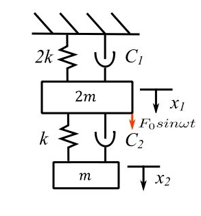
The equations of motion are:
![\[\begin{bmatrix}2m && 0 \\ 0 && m \end{bmatrix} \begin{Bmatrix} \Ddot{x}_1 \\ \Ddot{x}_2 \end{Bmatrix} + \begin{bmatrix} 3k && -k \\ -k && k \end{bmatrix} \begin{Bmatrix} x_1 \\ x_2 \end{Bmatrix} + \begin{bmatrix} c_1+c_2 && -c_2 \\ -c_2 && c_2 \end{bmatrix} \begin{Bmatrix} \dot{x}_1 \\ \dot{x}_2 \end{Bmatrix} = \begin{Bmatrix} F_0\sin{\omega t} \\ 0 \end{Bmatrix}\]](https://engcourses-uofa.ca/wp-content/ql-cache/quicklatex.com-d1580b4e4304a840a9dbd48b5f7c4e82_l3.png "Rendered by QuickLaTeX.com")
Consider the undamped problem to find the  and
and 
![\[ \begin{split}(3k-2mp^2)(k-mp^2)-k^2 &= 0 \\p^4-\frac{5}{2}\frac{k}{m}p^2 + \frac{k^2}{m^2} &= 0\end{split}\]](https://engcourses-uofa.ca/wp-content/ql-cache/quicklatex.com-f96a9097de0d9270f01c29a31bfc2baf_l3.png "Rendered by QuickLaTeX.com")
therefore:
![\[ p^2 = \frac{1}{2}\frac{k}{m}, \frac{2k}{m} \]](https://engcourses-uofa.ca/wp-content/ql-cache/quicklatex.com-8cdcdf248c76c935e1cf157b763754cc_l3.png "Rendered by QuickLaTeX.com")
![\[ (3k - 2mp^2)u_1 - ku_2 = 0 \]](https://engcourses-uofa.ca/wp-content/ql-cache/quicklatex.com-3285d9329a4b188e7b9b6fa8c0b5cf6b_l3.png "Rendered by QuickLaTeX.com")
therefore:
![\[ \begin{split}\frac{u_2}{u_1} &= 3-\frac{2m}{k}p^2 \\\biggr( \frac{u_2}{u_1} \biggr)_1 &= 2 \\\biggr( \frac{u_2}{u_1} \biggr)_2 &= -1 \\\end{split} \]](https://engcourses-uofa.ca/wp-content/ql-cache/quicklatex.com-ff3d70ab655bf410114c75f257ae4bb9_l3.png "Rendered by QuickLaTeX.com")
![\[ \begin{split}\begin{Bmatrix} u \end{Bmatrix}_1 &= \begin{Bmatrix} 1 \\ 2 \end{Bmatrix} \\\begin{Bmatrix} u \end{Bmatrix}_2 &= \begin{Bmatrix} 1 \\ -1 \end{Bmatrix}\end{split} \]](https://engcourses-uofa.ca/wp-content/ql-cache/quicklatex.com-e883bb979106585450a22cdcada0b91c_l3.png "Rendered by QuickLaTeX.com")
To find 
![\[ m \alpha_1^2 \begin{bmatrix} 1 && 2 \end{bmatrix} \begin{bmatrix} 2 && 0 \\ 0 && 1 \end{bmatrix} \begin{bmatrix} 1 \\ 2 \end{bmatrix} = 1 \]](https://engcourses-uofa.ca/wp-content/ql-cache/quicklatex.com-886b02293dde75b538aacefdc08c77bb_l3.png "Rendered by QuickLaTeX.com")
Therefore 
In the same manner, 
Therefore:
![\[ \begin{split}\begin{bmatrix} \mu \end{bmatrix} &= \frac{1}{\sqrt{6m}}\begin{bmatrix} 1 && \sqrt{2} \\ 2 && -\sqrt{2} \end{bmatrix} \\\begin{bmatrix} \mu \end{bmatrix}^T \begin{Bmatrix} F_0\sin{\omega t} \\ 0 \end{Bmatrix}&= \frac{\sin{\omega t}}{\sqrt{6m}} \begin{Bmatrix} F_0 \\ \sqrt{2}F_0 \end{Bmatrix}\end{split} \]](https://engcourses-uofa.ca/wp-content/ql-cache/quicklatex.com-3f8a8ab309c2524ada53d42636e05ae8_l3.png "Rendered by QuickLaTeX.com")
Therefore undamped differential equations are
![\[ \begin{split}\Ddot{\eta}_1 + p_1^2\eta_1 &= \frac{F_0}{\sqrt{6m}}\sin{\omega t} \\\Ddot{\eta}_2 + p_2^2\eta_2 &= \frac{\sqrt{2}F_0}{\sqrt{6m}}\sin{\omega t}\end{split} \]](https://engcourses-uofa.ca/wp-content/ql-cache/quicklatex.com-e2362cc0f1ae91698f833320393d1ad0_l3.png "Rendered by QuickLaTeX.com")
The undamped steady state solution is
![\[ \begin{split}\eta_1 &= \frac{F_0}{\sqrt{6m}}\frac{\sin{\omega t}}{(p_1^2-\omega^2)} \\\eta_2 &= \frac{\sqrt{2}F_0}{\sqrt{6m}}\frac{\sin{\omega t}}{(p_2^2-\omega^2)}\end{split} \]](https://engcourses-uofa.ca/wp-content/ql-cache/quicklatex.com-7125d1cc9f6addbfd610a6143a465661_l3.png "Rendered by QuickLaTeX.com")
As a result the undamped solution is
![\[ \begin{bmatrix} x \end{bmatrix} = \begin{bmatrix} \mu \end{bmatrix} \begin{Bmatrix} \eta \end{Bmatrix} \]](https://engcourses-uofa.ca/wp-content/ql-cache/quicklatex.com-0b20b8a863534d54bcb2ebd2457f0175_l3.png "Rendered by QuickLaTeX.com")
![\[ \begin{split}x_1 &= \frac{1}{\sqrt{6m}}\biggr[ \eta_1 + \sqrt{2}\eta_2 \biggr] \\x_2 &= \frac{1}{\sqrt{6m}}\biggr[ 2\eta_1 - \sqrt{2}\eta_2 \biggr]\end{split} \]](https://engcourses-uofa.ca/wp-content/ql-cache/quicklatex.com-98529d0884d146ff4694326a67993365_l3.png "Rendered by QuickLaTeX.com")
![\[ \begin{split}x_1 &= \frac{F_0\sin{\omega t}}{6m}\biggr[ \frac{1}{(p_1^2-\omega^2)} + \frac{2}{(p_2^2-\omega^2)} \biggr] \equiv X_1\sin{\omega t} \\x_2 &= \frac{F_0\sin{\omega t}}{6m}\biggr[ \frac{2}{(p_1^2-\omega^2)} - \frac{2}{(p_2^2-\omega^2)} \biggr] \equiv X_2\sin{\omega t}\end{split} \]](https://engcourses-uofa.ca/wp-content/ql-cache/quicklatex.com-8ab354e1278c4ce988a45acdb93fa3b7_l3.png "Rendered by QuickLaTeX.com")
![\[ \begin{split}X_1 &= \frac{F_0}{6m}\biggr[ \frac{(p^2_2-\omega^2) + 2(p_1^2-\omega^2)}{(p_1^2 - \omega^2)(p_2^2 - \omega^2)} \biggr] \\&= \frac{F_0}{2k} \frac{[\frac{k}{m} - \omega^2 ]}{ (p_1^2-\omega^2) (p^2_2-\omega^2)}\end{split} \]](https://engcourses-uofa.ca/wp-content/ql-cache/quicklatex.com-e52fe46f94355a141d5baa695779ca7d_l3.png "Rendered by QuickLaTeX.com")
![\[ X_2 = \frac{F_0}{2k}\frac{[\frac{k}{m}]}{(p_1^2-\omega^2)(p_2^2-\omega^2)} \]](https://engcourses-uofa.ca/wp-content/ql-cache/quicklatex.com-3c62ea5b078e6ae286dfd4308c149ef1_l3.png "Rendered by QuickLaTeX.com")
As was shown previously at 
![\[ \begin{split}X_1 &= 0 \\X_2 &= -\frac{F_0}{k}\end{split} \]](https://engcourses-uofa.ca/wp-content/ql-cache/quicklatex.com-ebde9b6b62388f474b0170b0daaf2e37_l3.png "Rendered by QuickLaTeX.com")
Now lets add damping
![\[ \begin{split}\begin{bmatrix} \mu \end{bmatrix}^T \begin{bmatrix} c \end{bmatrix} \begin{bmatrix} \mu \end{bmatrix} &= \frac{1}{6m} \begin{bmatrix} 1 && 2 \\ \sqrt{2} && -\sqrt{2} \end{bmatrix} \begin{bmatrix} c_1+c_2 && -c_2 \\ -c_2 && c_2 \end{bmatrix} \begin{bmatrix} 1 && \sqrt{2} \\ 2 && -\sqrt{2} \end{bmatrix} \\&= \frac{1}{6m} \begin{bmatrix} c_1+c_2(3-\sqrt{2}) && \sqrt{2}c_1-2\sqrt{2}c_2 \\ \sqrt{2}c_1-2\sqrt{2}c_2 && 2c_1 \end{bmatrix}\end{split} \]](https://engcourses-uofa.ca/wp-content/ql-cache/quicklatex.com-61948a709d0e4a8db542fbd36dd8a5ac_l3.png "Rendered by QuickLaTeX.com")
Therefore:
![\[ \begin{split}c_1 &= 2c_2 \\ &= 2c \\ c_2 &= c\end{split} \]](https://engcourses-uofa.ca/wp-content/ql-cache/quicklatex.com-439c3cc97854884928819be8f6168a20_l3.png "Rendered by QuickLaTeX.com")
![\[ \begin{split}\begin{bmatrix} \mu \end{bmatrix}^T \begin{bmatrix} c \end{bmatrix} \begin{bmatrix} \mu \end{bmatrix} &= \frac{1}{6m} \begin{bmatrix} (5-\sqrt{2})c && 0 \\ 0 && 2c \end{bmatrix} \\ &= \frac{1}{6m} \begin{bmatrix} \hat{c}_1 && 0 \\ 0 && \hat{c}_2 \end{bmatrix}\end{split} \]](https://engcourses-uofa.ca/wp-content/ql-cache/quicklatex.com-b6e3115d1bcfa99f6d28f00b061e5f76_l3.png "Rendered by QuickLaTeX.com")
Therefore the equations of motion are:
![\[ \begin{split}\Ddot{\eta}_1 + p_1^2 \eta_1 + \frac{\hat{c}_1}{6m} \dot{\eta}_1 &= \frac{F_0}{\sqrt{6m}} \sin{\omega t} \\\Ddot{\eta}_2 + p_2^2 \eta_2 + \frac{\hat{c}_2}{6m} \dot{\eta}_1 &= \frac{\sqrt{2}F_0}{\sqrt{6m}} \sin{\omega t} \\\end{split} \]](https://engcourses-uofa.ca/wp-content/ql-cache/quicklatex.com-5699c43cef828b19cbf9ef8b33588a54_l3.png "Rendered by QuickLaTeX.com")
Consider the standard form where the coefficient of  is
is 
![\[ \frac{\hat{c}_1}{6m} = 2\nu_1p_1 \]](https://engcourses-uofa.ca/wp-content/ql-cache/quicklatex.com-9d9c9d484ce71effcd4f145de285e526_l3.png "Rendered by QuickLaTeX.com")
Therefore
![\[ \begin{split}\nu_1 &= \frac{\hat{c}_1}{12mp_1} \\&= \frac{(5-\sqrt{2})c}{12mp_1} \\\nu_2 &= \frac{c}{6mp_2}\end{split} \]](https://engcourses-uofa.ca/wp-content/ql-cache/quicklatex.com-5799562d57e72958d514fe4421fdbf7c_l3.png "Rendered by QuickLaTeX.com")