
Review of single and multi-degree of freedom (mdof) systems: Complex Representation for Vibrations
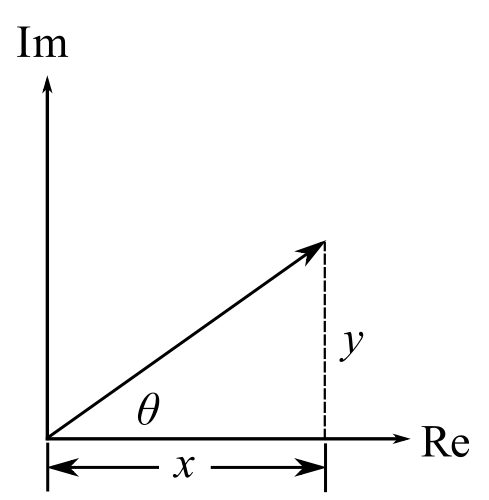
When dealing with vibrating equations it is often more efficient to use complex numbers as they allow the phase relationships to be easily handled. To do this use the complex number:
![\[ z = x + iy,\ i = \sqrt -1 \]](https://engcourses-uofa.ca/wp-content/ql-cache/quicklatex.com-8852ed3ffb2130623c7262496e592033_l3.png "Rendered by QuickLaTeX.com")
![\[ x = Re(z),\ y = Im(z) \]](https://engcourses-uofa.ca/wp-content/ql-cache/quicklatex.com-1a39d75233eb174afb755941b1174cc4_l3.png "Rendered by QuickLaTeX.com")
 is called the complex conjugate
![\[ z z ^ \star = x^2 + y^2 = |z |^2 \]](https://engcourses-uofa.ca/wp-content/ql-cache/quicklatex.com-ec9eaa6920d18c11049f5663e642b4c9_l3.png "Rendered by QuickLaTeX.com")
Alternatively we write  as:
as:
![\[ z = |z|e^{i\theta}, \theta = \tan^{-1}\Big(\frac{y}{x}\Big) \]](https://engcourses-uofa.ca/wp-content/ql-cache/quicklatex.com-7298ca8e33e89c79dffa4ae548ab5c13_l3.png "Rendered by QuickLaTeX.com")
 is called a unit phasor. For fractional expressions we can rationalize the denominator to separate real & imaginary parts:
![\[ C = \frac{A}{B} = \frac{a + i\alpha}{b+i\beta} , C^\star = \frac{a - i\alpha}{b- i\beta} \]](https://engcourses-uofa.ca/wp-content/ql-cache/quicklatex.com-b38b2c15f7b283c4d2da4fdca9dd9707_l3.png "Rendered by QuickLaTeX.com")
![\[ \begin{split} C &= \frac{a + i\alpha}{b+i\beta} \frac{b- i\beta}{b- i\beta} \\&= \frac{(ab+\alpha \beta ) + i(\alpha b - a \beta)}{b^2 + \beta ^2} \end{split} \]](https://engcourses-uofa.ca/wp-content/ql-cache/quicklatex.com-fb3939b74b9d558b84b7694209e8078c_l3.png "Rendered by QuickLaTeX.com")
![\[ \begin{split} C^\star &= \frac{a - i\alpha}{b-i\beta} \frac{b+ i\beta}{b+ i\beta} \\&= \frac{(ab+\alpha \beta ) - i(\alpha b - a \beta)}{b^2 + \beta ^2} \end{split} \]](https://engcourses-uofa.ca/wp-content/ql-cache/quicklatex.com-71b8ab3bc66d2016a75db65a352a4daf_l3.png "Rendered by QuickLaTeX.com")
Consider the steady-state forced SDOF system:
![\[ m \ddot{{x}} + c \dot{x} + kx = F_o \sin\omega t \]](https://engcourses-uofa.ca/wp-content/ql-cache/quicklatex.com-fe5f2bf0c0a34d551a924ac2b81cdb54_l3.png "Rendered by QuickLaTeX.com")
![\[ m \ddot{\tilde{x}} + c \dot{\tilde{x}} + k \tilde{x} = F_o e^{i \omega t} \]](https://engcourses-uofa.ca/wp-content/ql-cache/quicklatex.com-7c475e81776eb1aba7a83c5784e88609_l3.png "Rendered by QuickLaTeX.com")
and we want to imaginary part of the solution
Try  , where
  is complex, therefore:
![\[ (-m\omega ^2 \tilde{X} +ic \omega \tilde{X} + k \tilde{X})e^{i \omega t} = F_o e^{i \omega t} (\star) \]](https://engcourses-uofa.ca/wp-content/ql-cache/quicklatex.com-ff10fde1701a0b5a128529c743debc8d_l3.png "Rendered by QuickLaTeX.com")
![\[ \tilde{X} = \frac{F_o}{(k-m \omega ^2) + ic \omega} \]](https://engcourses-uofa.ca/wp-content/ql-cache/quicklatex.com-9e200188808bc234117001a63dee3701_l3.png "Rendered by QuickLaTeX.com")
Note:  ,
,  is defined as the mechanical impedence.
Rationalizing the denominator gives:
![\[ \begin{split} \tilde{X} &= \frac{F_o [(k - m \omega ^2) - ic \omega]}{[(k - m \omega ^2) +(c \omega )^2]} \\& \equiv Xe^{-i \phi} \end{split} \]](https://engcourses-uofa.ca/wp-content/ql-cache/quicklatex.com-dade4481aa6aa284020ae7f06ec5f311_l3.png "Rendered by QuickLaTeX.com")
![\[ \begin{split} X &= |\tilde{X}| \\&=\frac{F_o}{\sqrt{(k-m \omega ^2)^2 + (c \omega)^2}} \end{split} \]](https://engcourses-uofa.ca/wp-content/ql-cache/quicklatex.com-f7b1acfe94bbe8af54de42d1ee6628d7_l3.png "Rendered by QuickLaTeX.com")
![\[ \phi = \tan^{-1}{\frac{c\omega}{(k-m \omega)^2} } \]](https://engcourses-uofa.ca/wp-content/ql-cache/quicklatex.com-ebf9ecffee3ab1848860033067acd011_l3.png "Rendered by QuickLaTeX.com")
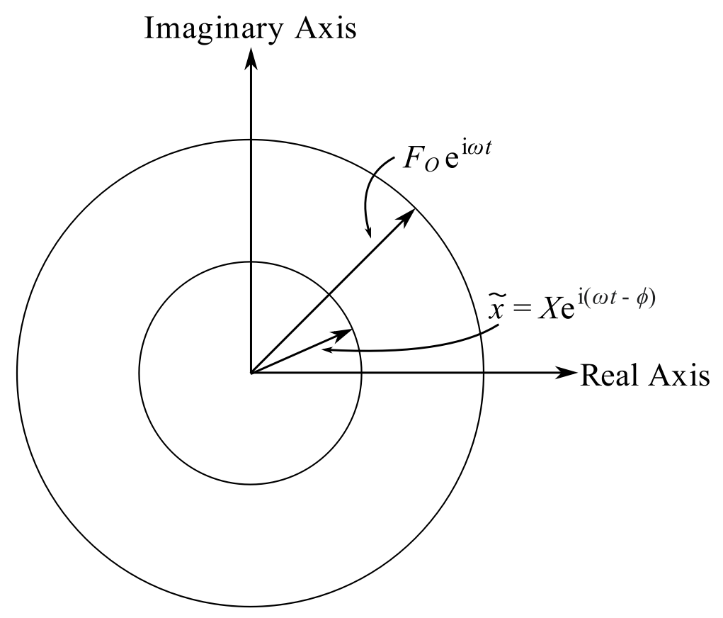
![\[ \begin{split} \tilde{x} &=\frac{F_o}{\sqrt{(k-m \omega ^2)^2 + (c \omega)^2}} e\strut^{-i\phi} e\strut^{i \omega t} \\ &= Xe\strut^{i(\omega t - \phi)} \end{split} \]](https://engcourses-uofa.ca/wp-content/ql-cache/quicklatex.com-5aad72d216c474e58b80115bada77e91_l3.png "Rendered by QuickLaTeX.com")
as 
Then the imaginary part of the solution is:
![\[ x(t) = \frac{F_o}{\sqrt{ (k-m \omega ^2)^2 + (c \omega)^2}} \sin(\omega t - \phi) \]](https://engcourses-uofa.ca/wp-content/ql-cache/quicklatex.com-2a862d25808625c348300fb6e60a359b_l3.png "Rendered by QuickLaTeX.com")
We can now re-interpret equation  as:
as:
![\[ -m\omega ^2 \tilde{X}e^{i\omega t} + ic\omega \tilde{X} e^{i\omega t} + k \tilde{X}e^{i\omega t} = F_o e^{i\omega t} \]](https://engcourses-uofa.ca/wp-content/ql-cache/quicklatex.com-ce5fd7426f6dd649caa27526a7487b2a_l3.png "Rendered by QuickLaTeX.com")
![\[ m\omega ^2 \tilde{X}e^{i\pi}e^{i\omega t} +c \omega \tilde{X}e^{\frac{i\pi}{2}}e^{i\omega t} + k \tilde{X}e^{i \omega t} = F_o e^{i \omega t} \]](https://engcourses-uofa.ca/wp-content/ql-cache/quicklatex.com-c31e449edd09a4296755fd5a097702f8_l3.png "Rendered by QuickLaTeX.com")
Each of the force terms above can be interpreted in their respective phases.
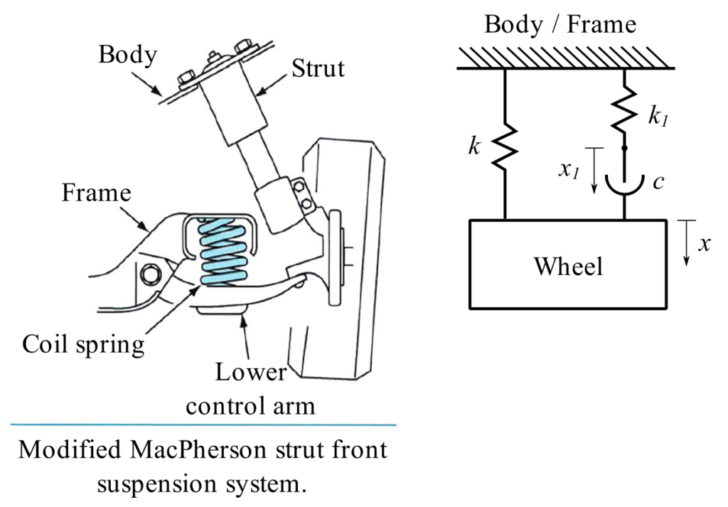
Many real automotive suspension systems use the so-called Macpherson strut which is a combined spring and damper along with a coil spring as shown in the diagram. The system can be represented by the diagram where the forcing function comes from road surface. (This system is sometimes called a 1 &  DOF system).
a) Using the mechanical impedance find that the displacement  and
and  .
.
b) For the model shown, determine the transmissibility of the system.
c) For the frequency ratio  , and for
  . Calculate for the transmissibility and compare the values to the case in which
  .
.
a)
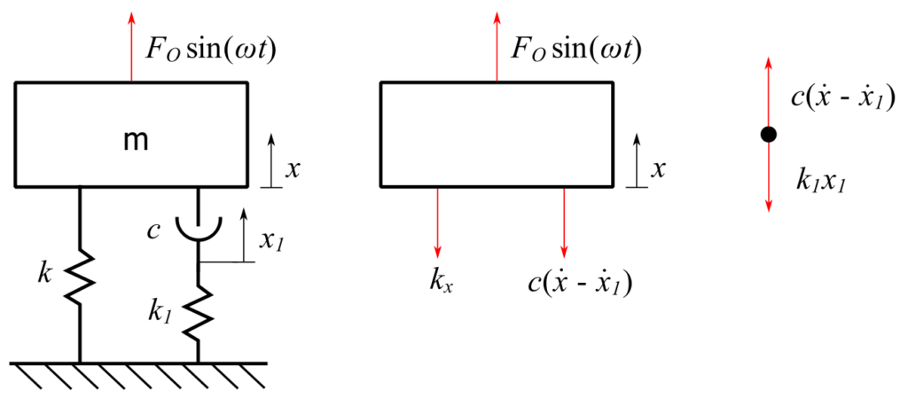
![\[ m \ddot{{x}} + c \dot{x} + kx - c\dot{x_1}= F_o \sin\omega t --- (1) \]](https://engcourses-uofa.ca/wp-content/ql-cache/quicklatex.com-00ea91bc902982d4dd19448c263262ec_l3.png "Rendered by QuickLaTeX.com")
![\[-c\dot{x} + c\dot{x_1} + k_1x_1 = 0 ---(2) \]](https://engcourses-uofa.ca/wp-content/ql-cache/quicklatex.com-384dff623df7ceae84c9eca79d6b7618_l3.png "Rendered by QuickLaTeX.com")
Using 

![\[ \begin{split} \hat{\Delta} &= (ms^2 +cs +k)(cs+ k_1) - c^2s^2 \\&= k_1(k+ms^2)+ cs(k+k_1+ms^2) \end{split} \]](https://engcourses-uofa.ca/wp-content/ql-cache/quicklatex.com-24b5e4fcf070ecc53c67c43e89d670f5_l3.png "Rendered by QuickLaTeX.com")
(3) is of the form:

Therefore:
![\[ \hat{X} =\frac{V_{22}(s)}{\hat{\Delta}}F \]](https://engcourses-uofa.ca/wp-content/ql-cache/quicklatex.com-ccd0d4c478c005cbf693d9a62f326eb8_l3.png "Rendered by QuickLaTeX.com")
![\[ \hat{X_1} = \frac{V_{12}(s)}{\hat{\Delta}}F \]](https://engcourses-uofa.ca/wp-content/ql-cache/quicklatex.com-5780f2b03141dce7977e6a398a564698_l3.png "Rendered by QuickLaTeX.com")
If  :
:
![\[ \hat{z} = \frac{(k_1 + ic \omega)}{\hat{\Delta}}F \]](https://engcourses-uofa.ca/wp-content/ql-cache/quicklatex.com-fce8973ce76045a94c8412e03d5a35b5_l3.png "Rendered by QuickLaTeX.com")
![\[ \hat{z_1} = \frac{ic\omega F}{\hat{\Delta}} \]](https://engcourses-uofa.ca/wp-content/ql-cache/quicklatex.com-9ca7e00920e7e84f88df3f0d9fd739e7_l3.png "Rendered by QuickLaTeX.com")
![\[ \frac{\hat{\Delta}}{kk_1} = \biggr[\Big(1- \frac{\omega^2}{p^2}\Big) + \frac{i\omega c}{k}\Big(1+\frac{1}{N} - \frac{\omega^2}{p^2N}\Big)\biggr] \]](https://engcourses-uofa.ca/wp-content/ql-cache/quicklatex.com-6d4ba9aceedf2e2077f8af7920192354_l3.png "Rendered by QuickLaTeX.com")
 , if
, if  :
:
![\[ \begin{split} \frac{\hat{\Delta}}{kk_1} &= \biggr[(1- r^2) + i2\zeta r\Big(1+\frac{1}{N} - \frac{r^2}{N}\Big)\biggr] \\&= \biggr[(1- r^2)^2 + \Big\{ 2\zeta r\Big(1+\frac{1}{N} - \frac{r^2}{N}\Big) \Big\}\strut^2\biggr]\strut^\frac{1}{2} e\strut^{i\gamma} \\&= \hat{\Delta}e\strut^{i\gamma} \end{split} \]](https://engcourses-uofa.ca/wp-content/ql-cache/quicklatex.com-ef8be54b3728d76a62178d104c8ad973_l3.png "Rendered by QuickLaTeX.com")
![\[ \gamma = \tan^{-1}(\frac{2\zeta r(1+\frac{1}{N} - \frac{r^2}{N})}{1-r^2}) \]](https://engcourses-uofa.ca/wp-content/ql-cache/quicklatex.com-cc60d6267096cf0a344e80f560a4bc61_l3.png "Rendered by QuickLaTeX.com")
If we set  ,
,
![\[ \begin{split} \hat{X} &= \frac{F(1+\frac{i2\zeta r}{N})}{k \Delta e\strut^{i\gamma}} \\ &= \frac{F \sqrt{(1+\frac{2\zeta r}{N})}e\strut^{i\beta}}{k \Delta e\strut^{i\gamma}} \end{split} \]](https://engcourses-uofa.ca/wp-content/ql-cache/quicklatex.com-494db35c245bc69f8fb5f3051fdda93a_l3.png "Rendered by QuickLaTeX.com")
![\[ \beta = \tan^{-1} \frac{2\zeta r}{N} \]](https://engcourses-uofa.ca/wp-content/ql-cache/quicklatex.com-5177029f8c6d8ccbe1a781d452ddd34a_l3.png "Rendered by QuickLaTeX.com")
Therefore,
![\[ \hat{X} = \frac{F \sqrt{(1+\frac{i2\zeta r}{N})}e\strut^{-i\alpha}}{k \Delta } \]](https://engcourses-uofa.ca/wp-content/ql-cache/quicklatex.com-c290c578f60f79c6a764c4886f4ce383_l3.png "Rendered by QuickLaTeX.com")
Where 
![\[ \hat{X_1} = \frac{F}{k\Delta} \frac{2 \zeta r}{N}e^{-i \alpha _1} \]](https://engcourses-uofa.ca/wp-content/ql-cache/quicklatex.com-61e01b13e91633aff5905cc55d5c6ca3_l3.png "Rendered by QuickLaTeX.com")
Where 
b) The force transmitted is
![\[ \begin{split} F_T &= k \hat{X} + k_1 \hat{X_1} \\ &= F \frac{[k(k_1+ic \omega ) + k_1(ic \omega )]}{\hat{\Delta}} \\&= kk_1 F \frac{[1 + \frac{ic\omega }{k} + \frac{ic\omega }{k_1}]}{\hat{\Delta}}\\&= F \frac{[1+ i(2 \zeta r + \frac{2\zeta r)}{N}]}{\hat{\Delta}e\strut^{i\gamma}} \\&= F \sqrt {1+ \big[2\zeta r\big(1+ \frac{1}{N}\big)\big]\strut^2} \frac{e\strut^{-i\alpha _2}}{\hat{\Delta}} \end{split} \]](https://engcourses-uofa.ca/wp-content/ql-cache/quicklatex.com-3d93db365b9bc67202077bbd7ff63eb3_l3.png "Rendered by QuickLaTeX.com")
![\[ \alpha _2 = \gamma - \tan^{-1}\biggr[2\zeta r\Big(1+\frac{1}{N}\Big)\biggr] \]](https://engcourses-uofa.ca/wp-content/ql-cache/quicklatex.com-e98fc2eb96533996876e07fa61b01c44_l3.png "Rendered by QuickLaTeX.com")
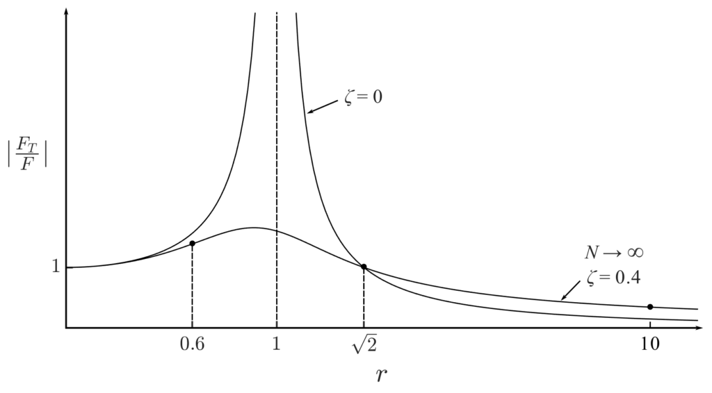
c) For the case  :
:
![\[ \left| \frac{F_T}{F} \right| = 1.37 \]](https://engcourses-uofa.ca/wp-content/ql-cache/quicklatex.com-7b8f10d678c24c057d5e1c977de3cf6a_l3.png "Rendered by QuickLaTeX.com")
![\[ \left| \frac{F_T}{F} \right| = 1.39 (k \rightarrow \infty) \]](https://engcourses-uofa.ca/wp-content/ql-cache/quicklatex.com-8595a6bde041a60d476bcf942aca8de8_l3.png "Rendered by QuickLaTeX.com")
For the case  :
:
![\[ \left| \frac{F_T}{F} \right| = 0.03 \]](https://engcourses-uofa.ca/wp-content/ql-cache/quicklatex.com-168aea436d1cac140329d3b503b88a8d_l3.png "Rendered by QuickLaTeX.com")
![\[ \left| \frac{F_T}{F} \right| = 0.081 (k \rightarrow \infty) \]](https://engcourses-uofa.ca/wp-content/ql-cache/quicklatex.com-346eb6c648743eb844f544dada4984f9_l3.png "Rendered by QuickLaTeX.com")
The added spring  reduces the transmissivity in both cases, however it is most effective at higher
  ratio.
![\[ \left| \frac{F_T}{F} \right| = \frac{\big[1+\{2\zeta r (1+ \frac{1}{N})\}^2\big]\strut^{1/2}}{\big[(1-r^2)^2+\{2\zeta r(1+\frac{1}{N} - \frac{r^2}{N}\}^2\big]\strut^{1/2}} \]](https://engcourses-uofa.ca/wp-content/ql-cache/quicklatex.com-d1cd721cbf3a2d4fec75bfd2517c2100_l3.png "Rendered by QuickLaTeX.com")
If 
![\[ \left| \frac{F_T}{F} \right| = \frac{\big[1+(2 \zeta r)^2\big]\strut^{1/2}}{\big[(1-r^2)^2+(2\zeta r)^2\big]\strut^{1/2}} \]](https://engcourses-uofa.ca/wp-content/ql-cache/quicklatex.com-a2a51c7432c957ee4ecdaccb56f0e6c6_l3.png "Rendered by QuickLaTeX.com")
![\[ r = 0.6, N = 2, \zeta = 0.4 \]](https://engcourses-uofa.ca/wp-content/ql-cache/quicklatex.com-cf5df2b351df3fb850c55cc759aefb33_l3.png "Rendered by QuickLaTeX.com")
![\[ \left| \frac{F_T}{F} \right| = \frac{\big[1+\{2(0.4)(0.6)\frac{3}{2}\}^2\big]\strut^{1/2}}{\big[(1-0.36)^2+\{2(0.4)(0.6)(1+\frac{1}{2} - 0.18)\}^2\big]\strut^{1/2}} \]](https://engcourses-uofa.ca/wp-content/ql-cache/quicklatex.com-6cebd3fdbe57b26c44d9359207c29f2a_l3.png "Rendered by QuickLaTeX.com")
![\[ = \underline{\underline{1.37}} \]](https://engcourses-uofa.ca/wp-content/ql-cache/quicklatex.com-6db545b0d1828fac02f5aa7161fe281a_l3.png "Rendered by QuickLaTeX.com")
![\[ \frac{|F_T|}{F}\Bigg|_{k \rightarrow \infty} = \underline{\underline{1.39}} \]](https://engcourses-uofa.ca/wp-content/ql-cache/quicklatex.com-51b69f4f2377cab03375dec8de34ce68_l3.png "Rendered by QuickLaTeX.com")
![\[ r = 10, N = 2, \zeta = 0.4 \]](https://engcourses-uofa.ca/wp-content/ql-cache/quicklatex.com-12795950944113fbac0e7beee57b2652_l3.png "Rendered by QuickLaTeX.com")
![\[ \left| \frac{F_T}{F} \right| = \frac{\big[1+\{2(0.4)(10)\frac{3}{2}\}^2\big]\strut^{1/2}}{\big[(1-10^2)^2+\{2(0.4)(10)(\frac{3}{2} - \frac{100}{2})\}^2\big]\strut^{1/2}} \]](https://engcourses-uofa.ca/wp-content/ql-cache/quicklatex.com-2df671ac3fe73134549349bba2f88ace_l3.png "Rendered by QuickLaTeX.com")
![\[ = \underline{\underline{0.032}} \]](https://engcourses-uofa.ca/wp-content/ql-cache/quicklatex.com-94a429e8c22c1101602a1a3d80e87c02_l3.png "Rendered by QuickLaTeX.com")
![\[ \frac{|F_T|}{F}\Bigg|_{k \rightarrow \infty} = \frac{\big[1+\{2(0.4)(10)\}^2\big]\strut^{1/2}}{\big[(1-10^2)^2+\{2(0.4)(10)\}^2\big]\strut^{1/2}} \]](https://engcourses-uofa.ca/wp-content/ql-cache/quicklatex.com-0f63abcb8196336c9b4cb882607f49b0_l3.png "Rendered by QuickLaTeX.com")
![\[ = \frac{8.062}{99.32} \]](https://engcourses-uofa.ca/wp-content/ql-cache/quicklatex.com-e6eaf098f4398d1627f9b6ea5d5709cf_l3.png "Rendered by QuickLaTeX.com")
![\[ = \underline{\underline{0.081}} \]](https://engcourses-uofa.ca/wp-content/ql-cache/quicklatex.com-57331e7efc9a49b670a337951fbe9f99_l3.png "Rendered by QuickLaTeX.com")
Extra Details
![\[ \begin{split} \hat{\Delta} &= (ms^2 + cs + k)(cs + k_1) - c^2s^2 \\ &= cs(ms^2+k+k_1)+c^2s^2+k_1(k+ms^2)-c^2s^2 \\ &= cs(ms^2+k+k_1) + k_1(k+ms^2) \end{split} \]](https://engcourses-uofa.ca/wp-content/ql-cache/quicklatex.com-7dc3a93462ab2834e395269a97f69e79_l3.png "Rendered by QuickLaTeX.com")
If  :
:
 \]](https://engcourses-uofa.ca/wp-content/ql-cache/quicklatex.com-4c9138201e3c7d885d51dd749d7331c3_l3.png "Rendered by QuickLaTeX.com")
![\[ \begin{split} \frac{\hat{\Delta}}{kk_1} &= \Big[1 - \frac{\omega^2m}{k}\Big] + \frac{ic\omega}{k}\Big[\frac{-m\omega^2}{k_1} + 1 + \frac{k}{k_1}\Big] \\ &= \Big[1 - \frac{\omega^2}{p^2}\Big] + \frac{ic\omega m}{k}\Big[1 + \frac{1}{N} - \frac{r^2}{N}\Big] \end{split} \]](https://engcourses-uofa.ca/wp-content/ql-cache/quicklatex.com-545e6731bd6da4a77bab7cba388f0ab4_l3.png "Rendered by QuickLaTeX.com")
Where  ,
,  , and
, and  . Thus:
![\[ \begin{split} &= [1-r^2] + i2\zeta r\Big[1 + \frac{1}{N} - \frac{r^2}{N}\Big] \\ &= \biggr\{[1-r^2]^2 + \Big(2\zeta r\Big(1 + \frac{1}{N} - \frac{r^2}{N}\Big)\Big)^2\biggr\}\strut^{\frac{1}{2}}e\strut^{i\gamma} \end{split} \]](https://engcourses-uofa.ca/wp-content/ql-cache/quicklatex.com-8bf5fe117f7505f2355ca5720620e9e0_l3.png "Rendered by QuickLaTeX.com")
Where:
![\[ \gamma = \frac{\tan^{-1}(2\zeta r(1 + \frac{1}{N} - \frac{r^2}{N}))}{(1-r^2)} \]](https://engcourses-uofa.ca/wp-content/ql-cache/quicklatex.com-6d22e6f656e28e4c7253f226c5470706_l3.png "Rendered by QuickLaTeX.com")
If  ,
,  :
:
![\[ \begin{split} X &= \frac{\frac{F}{k}(1+\frac{2i\zeta r}{N})}{\Delta e^{i\zeta}} \\ &= \frac{\frac{F}{k}\sqrt{1 + (\frac{2\zeta r}{N})^2}}{\Delta e^{i\zeta}}e^{i\beta} \end{split} \]](https://engcourses-uofa.ca/wp-content/ql-cache/quicklatex.com-abe507540cf6712005fbf068ba57e6b6_l3.png "Rendered by QuickLaTeX.com")
![\[ \beta = \arctan{\frac{2\zeta r}{N}} \]](https://engcourses-uofa.ca/wp-content/ql-cache/quicklatex.com-8eba71fc04ac2a7d21397b684c325aec_l3.png "Rendered by QuickLaTeX.com")
![\[ X = \frac{F}{k\Delta}\sqrt{1 + (\frac{2\zeta r}{N})^2}e^{i\beta}e^{-i\gamma} \]](https://engcourses-uofa.ca/wp-content/ql-cache/quicklatex.com-0a1f7dda6639e4a492cf83ade2514e45_l3.png "Rendered by QuickLaTeX.com")
![\[ \equiv \underline{\underline{\frac{F}{k\Delta}\sqrt{1 + (\frac{2\zeta r}{N})^2}e^{i\alpha}} } \]](https://engcourses-uofa.ca/wp-content/ql-cache/quicklatex.com-ac9e2843eb5feb558484495c231657b7_l3.png "Rendered by QuickLaTeX.com")
![\[ \begin{split} X_1 &= \frac{ic\omega F}{\hat{\Delta}} \\&= \frac{2\zeta r}{N \hat{\Delta}} e ^{i\frac{\pi}{2}} \\&=\frac{F}{k\Delta}\frac{2\zeta r}{N}e^{-i(\gamma-\frac{\pi}{2})}\end{split} \]](https://engcourses-uofa.ca/wp-content/ql-cache/quicklatex.com-2e79eb325045159ff35b5961d3a4b561_l3.png "Rendered by QuickLaTeX.com")