Introduction to Numerical Analysis: Ordinary Differential Equations

Ordinary Differential Equations (ODEs) are equations that relate the derivatives of one or more smooth functions with an independent variable . The term “ordinary” indicates that there is only one independent variable appearing in the equations.

Examples of Ordinary Differential Equations

ODEs appear naturally in almost all engineering applications. Here are some examples:

Newton’s Second Law of Motion

One of the most ubiquitously used ordinary differential equations is Newton’s second law of motion, which relates the second derivative of the position of a particle (i.e., the acceleration) to the applied force on the particle. The relationship has the form:

where is the mass of the particle. The time is the independent variable, while the dependent variable is the position . Newton’s equation adopts different forms depending on the application. For example, if the applied force is the combined action of gravity and a spring with a constant (Figure 1), then the equation has the form:

The explicit solution to this equation has the following form:

where and are constants that depend on the initial conditions of the problem. If the initial displacement and velocity are equal to zero, i.e., and , then, the explicit solution has the form:

The following code utilizes the built-in DSolve function in Mathematica to solve the above simple equations. Also, the Manipulate built-in function is used to visualize the effect of varying and on the resulting vibration of the system.

Clear[x, g, k, m]
(*General Solution*)
a = DSolve[m*x''[t] == m*g - k*x[t], x, t];
Print["General Solution="]
x = x[t] /. a[[1]]

(*Solution with initial velocity and displacement =0*)
Clear[m, g, x, k]
a = DSolve[{m*g - k*x[t] == m*x''[t], x[0] == 0, x'[0] == 0}, x, t];
Print["Solution with initial velocity and displacement =0"]
x = x[t] /. a[[1]]

Manipulate[g = 1;
 Graphics3D[{Cuboid[{-1, -1, -5}, {0, 0, (g*m - g*m*Cos[Sqrt[k/m]*t])/k}]}, Axes -> True, PlotRange -> {{-1, 0}, {-1, 0}, {-5, 2*5/1}},  AxesOrigin -> {0, 0, 0}, ViewVertical -> {0, 0, -1}], {t, 0, 4*Pi*Sqrt[5]}, {m, 1, 5}, {k, 1, 5}]

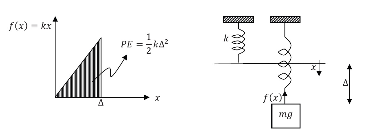
Figure 1. Mass – Linear Elastic Spring System

If the external forces include a damping force (a force that is a function of the velocity and that is always opposite to the direction of motion), then, the equation has the form:

where is the damping coefficient.
The explicit solution to this equation has the following form:

where and are constants that depend on the initial conditions of the problem. If the initial displacement and velocity are equal to zero, i.e., and , then, the explicit solution has the form:

The following code utilizes the built-in DSolve function in Mathematica to solve the above simple equations. Also, the Manipulate built-in function is used to visualize the effect of varying , , and on the resulting vibration of the system.

Clear[x, g, k, m]
(*General Solution*)
a = DSolve[m*x''[t] == m*g - k*x[t] - beta*x'[t], x, t];
Print["General Solution (damped system)="]
x = x[t] /. a[[1]]

(*Solution*)
Clear[x, g, k, m, beta]
a = DSolve[{m*x''[t] == m*g - k*x[t] - beta*x'[t], x[0] == 0, x'[0] == 0}, x, t];
Print["Solution with initial velocity and displacement =0"]
x = x[t] /. a[[1]];
x = Simplify[x]
Manipulate[g = 1;Graphics3D[{Cuboid[{-1, -1, -5}, {0, 0, -((E^(-(((beta + Sqrt[beta^2 - 4 k m]) t)/(2 m)))m (beta (-1 + E^((Sqrt[beta^2 - 4 k m] t)/m)) + (1 + E^((Sqrt[beta^2 - 4 k m] t)/m)-2 E^(((beta + Sqrt[beta^2 - 4 k m]) t)/(2 m))) Sqrt[beta^2 - 4 k m]))/(2 k Sqrt[beta^2 - 4 k m]))}]},  Axes -> True, PlotRange -> {{-1, 0}, {-1, 0}, {-5, 10}},  AxesOrigin -> {0, 0, 0}, ViewVertical -> {0, 0, -1}], {t, 0,  2*4*Pi*Sqrt[5]}, {m, 1, 5}, {beta, 0, 5}, {k, 1, 5}]

Beam Deflection

The deflection of an Euler-Bernoulli beam follows the following equation:

where is the beam’s Young’s modulus, is the cross sectional moment of inertia, is the beam’s deflection (the dependent variable), is the applied distributed load on the beam, and is the position along the beam’s length (the independent variable). For a fixed-ends beam; if the deflection and rotation at both ends of a beam of length is equal to zero, i.e. , and if is constant, then, the deflection of the beam has the form:

Growth and Decay

If is the number of organisms at any time , and if the growth of the number depends on the number that is already there, then, the ODE that would describe this uninhibited growth is given by:

Where is a positive constant. The time is the independent variable, while the dependent variable is the number of organisms . The general solution of this equation has the form:

where is a constant depending on the boundary conditions. If the initial condition is such that then, the solution has the form:

Similarly, if rate of decrease (decay) of a quantity is a function of the amount available, then, the uninhibited decay can be described by the equation:

where is a positive constant. The time is the independent variable, while the dependent variable is the quantity . Radioactive decay follows this ODE. The general solution of this equation has the form:

where is a constant depending on the boundary conditions. If the initial condition is such that then, the solution has the form:

The following tool plots the quantities or when for different values of the exponent:

Clear[x]
a = DSolve[x'[t] == k*x[t], x, t];
x = x[t] /. a[[1]]

Clear[x]
a = DSolve[{x'[t] == k*x[t], x[0] == A}, x, t]
x = x[t] /. a[[1]]

Manipulate[A = 1; r = Grid[{{"k=", k}}, Spacings -> 0]; Grid[{{Plot[A*E^(k*t), {t, 0, 20}, AxesLabel -> {"t", "x(t) or y(t)"}, ImageSize -> Medium]}, {r}}], {k, -0.5, 0.5}]

Electrical Capacitors and Inductors

Simple electric circuits are composed of three components: resistances, capacitors, and inductors. The relationship between the voltage drop across a resistance, and the current passing through it is given by:

where is the constant of proportionality, namely the value of the electric resistance. A capacitor on the other hand is an element that has the following relationship between the current passing through it and the rate of change of the voltage drop across it :

where is the constant of proportionality, namely the capacitance. An inductor is an element that has the following relationship between the voltage drop across it and the rate of change of the current that passes through it :

Where is the constant of proportionality, namely the inductance. When the elements are combined, ODEs are generated with being the independent variable, and and being the dependent variables.

Classification of ODEs

Order

The order of an ODE is the order of the highest derivative appearing in the equation. For example, the following equation (Newton’s equation) is a second-order ODE:

while the beam equation is a fourth-order ODE:

Linear vs. Nonlinear

An ODE is linear if it can be written as the linear combination:

where and are functions of the independent variable . All the examples above are considered linear ODEs.
The following are two examples of nonlinear ODEs with being the dependent variable and being the independent variable:

Homogeneous vs. Nonhomogeneous

A homogeneous ODE is an equation whose every term contains either the dependent variable or one of its derivatives. For example, Newton’s second law applied to a spring without the gravitational term is a linear homogeneous ODE:

If one of the non-zero terms in the ODE contains neither the dependent variable nor any of its derivatives, the equation is nonhomogeneous. As an example, if the gravitational term is added to Newton’s second law, then, the equation becomes nonhomogeneous:

The free term (the term devoid of the dependent variables and any of its derivatives) is called the source term.

A linear homogeneous ODE has the following form:

while a linear nonhomogeneous ODE has the form:

The term is called the source term. The solution to a linear homogeneous equation is called the complementary solution while the solution when a source term appears in the equation is the sum of the complementary solution and the particular solution (which is particular to the source term ). For example, the solution to Newton’s second law without the gravitational term has the form:

while the solution when the gravitational term appears has the form:

The particular solution is the term .

IVP vs. BVP

Depending on the boundary conditions, an ODE can be classified as either an Initial Value Problem (IVP) or a Boundary Value Problem (BVP). An initial value problem is an ODE given with initial conditions of the dependent variable and its derivative at a particular value of the independent variable. This usually applies to dynamic systems whose independent variable is time. For example, Newton’s second law of motion is an initial value problem because the initial value at of the displacement and the velocity are required to reach a solution. The initial values lead to a particular path that is a function of time .

A boundary value problem is an ODE given with boundary conditions at different points. This usually applies to static systems whose independent variable is position. For example, the Euler-Bernoulli beam deflection equation is a boundary value problem. The boundary conditions of the displacement , the rotation , and the third and fourth derivatives, are usually given at boundary points on the beam which will then dictate the equilibrium deflection of the beam as a function of position .

Solution Methods for IVPs

(Explicit) Euler Method

The Euler method is one of the simplest methods for solving first-order IVPs. Consider the following IVP:

Assuming that the value of the dependent variable (say ) is known at an initial value , then, we can use a Taylor approximation to estimate the value of at , namely with :

Substituting the differential equation into the above equation yields:

Therefore, as an approximation, an estimate for can be taken as as follows:

Using this estimate, the local truncation error is thus proportional to the square of the step size with the constant of proportionality related to the second derivative of , which is the first derivative of the given IVP:

If the errors from each interval are added together, with being the number of intervals and the total length , then, the total error is:

There are many examples in engineering and biology in which such IVPs appear. Check this page for examples.

The following Mathematica code provides a procedure whose inputs are

• The differential equation as a function of the dependent variable and the independent variable .
• The step size .
• The initial value and the final value of the independent variable.
• The initial value .

The procedure then carries on the Euler method and outputs the required data vector.
View Mathematica Code

EulerMethod[fp_, x0_, h_, t0_, tmax_] :=
 (n = (tmax - t0)/h + 1;
  xtable = Table[0, {i, 1, n}];
  xtable[[1]] = x0;
  Do[xtable[[i]] = xtable[[i - 1]] + h*fp[xtable[[i - 1]], t0 + (i - 2) h], {i, 2,  n}];
  Data = Table[{t0 + (i - 1)*h, xtable[[i]]}, {i, 1, n}];
  Data)
function1[y_, t_] := 0.05 y
function2[x_, t_] := 0.015 x
EulerMethod[function1, 35, 1.0, 0, 50] // MatrixForm
EulerMethod[function2, 35, 1.0, 0, 50] // MatrixForm

Example 1

The Canadian population at (current year) is 35 million. If 2.5% of the population have a child in a given year, while the death rate is 1% of the population, what will the population be in 50 years? What if 6% of the population have a child in a given year and the death rate is kept constant at 1%, what will the population be in 50 years?

Solution

The rate of growth is directly proportional to the current population with the constant of proportionality . If represents the population in millions and represents the time in years, then the IVP is given by:

With the initial condition of , the exact solution to this differential equation is:

If the birth rate is 6%, then and the exact solution of the population follows the following equation:

The Euler method provides a numerical solution as follows. Using a step size of , we can set years. The value of is given as 35 million. When , the value of in millions is given by:

The value of is given by:

Iterating further, the values of at each time point can be obtained. The following is the Microsoft Excel table showing the values of in years and the corresponding values of the population in millions:

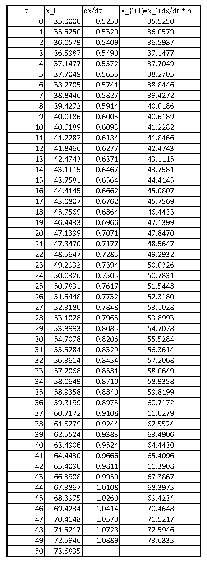
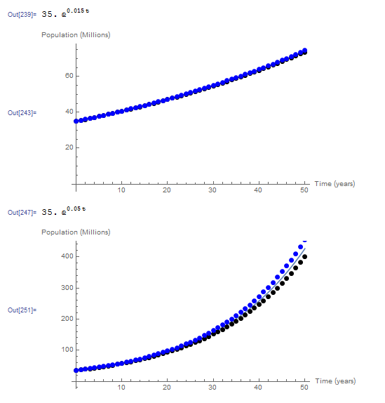
When , the numerical procedure produces a very good approximation for the population at years. The error between the prediction of the exact solution to the differential equation and the numerical value at is given in millions by:

The relative error in this case is given by:

For the second case, when , the value of in millions is given by:

Proceeding iteratively, the following is the Microsoft Excel table showing the values of in years and the corresponding values of the population in millions:

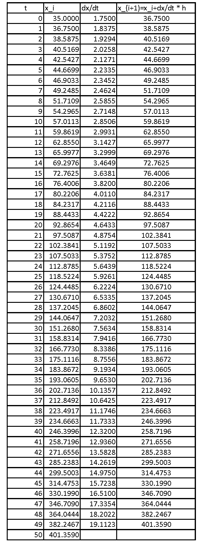
Compared to the previous case, when , the numerical procedure is not as good. The error between the prediction of the exact solution to the differential equation and the numerical value at is given in millions by:

The relative error in this case is given by:

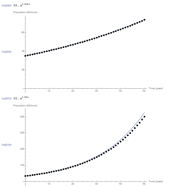
The following is the graph showing the exact solution versus the data using the Euler method for both cases. The Mathematica code used is given below. Notice how the error in the Euler method increases as increases.

View Mathematica Code

EulerMethod[fp_, x0_, h_, t0_, tmax_] := 
  (n = (tmax - t0)/h + 1;
  xtable = Table[0, {i, 1, n}];
  xtable[[1]] = x0;
  Do[xtable[[i]] =  xtable[[i - 1]] + h*fp[xtable[[i - 1]], t0 + (i - 2) h], {i, 2, n}];
  Data = Table[{t0 + (i - 1)*h, xtable[[i]]}, {i, 1, n}];
  Data)

Clear[x, xtable]
k = 0.015;
a = DSolve[{x'[t] == k*x[t], x[0] == 35}, x, t];
x = x[t] /. a[[1]]
fp[x_, t_] := k*x;
Data = EulerMethod[fp, 35, 1.0, 0, 50];
Plot[x, {t, 0, 50}, Epilog -> {PointSize[Large], Point[Data]}, AxesOrigin -> {0, 0}, AxesLabel -> {"Time (years)", "Population (Millions)"}]

Clear[x, xtable]
k = 0.05;
a = DSolve[{x'[t] == k*x[t], x[0] == 35}, x, t];
x = x[t] /. a[[1]]
fp[x_, t_] := k*x;
Data = EulerMethod[fp, 35, 1.0, 0, 50];
Plot[x, {t, 0, 50}, Epilog -> {PointSize[Large], Point[Data]}, AxesOrigin -> {0, 0}, AxesLabel -> {"Time (years)", "Population (Millions)"}]

The following tool illustrates the effect of choosing the step size on the difference between the numerical solution (shown as dots) and the exact solution (shown as the blue curve) for the case when . The smaller the step size, the more accurate the solution is. The higher the value of , the more the numerical solution deviates from the exact solution. The error increases away from the initial conditions.

Example 2

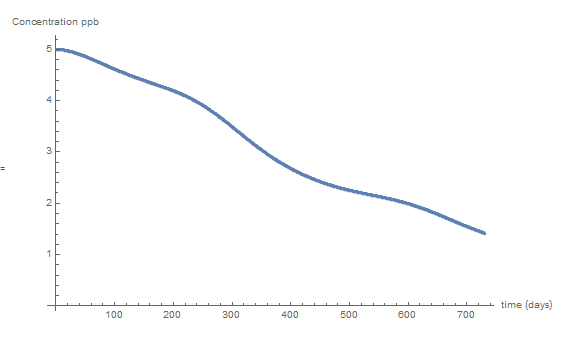
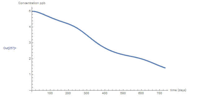
This example is adopted from this page. A lake of volume has an initial concentration of a particular pollutant of parts per billion (ppb). This pollutant is due to a pesticide that is no longer available in the market. The volume of the lake is constant throughout the year, with daily water flowing into and out of the lake at the rate of . As the pesticide is no longer used, the concentration of the pollutant in the surrounding soil is given in ppb as a function of (days) by which indicates that the concentration is following an exponential decay. This concentration can be assumed to be that of the pollutant in the fluid flowing into the lake. The concentration of the pollutant in the fluid flowing out of the lake is the same as the concentration in the lake. What is the concentration of this particular pollutant in the lake after two years?

Solution

The first step in this problem is to properly write the differential equation that needs to be solved. If is the total amount of pollutant in the lake, then, the rate of change of with respect to is equal to the total amount of pollutant entering into the lake per day. Each day, the total amount of pollutant entering the lake is given by , while the total amount of pollutant exiting the lake is given by . Therefore:

The concentration is equal to the total amount divided by the volume of the lake, therefore, the differential equation in terms of is given by:

Notice that finding an exact solution to the above differential equation is not an easy task and a numerical solution would be the preferred solution in this case. Taking day, , and ppb the Euler method can be used to find the concentration at days. You can download the Microsoft Excel file example2.xlsx showing the calculations and the produced graph.
Taking day, we will show the calculations for the estimates and . At day:

At days:

Carrying on produces the values of at the remaining time intervals up to days. The following is the output produced by the Mathematica code below.

EulerMethod[fp_, x0_, h_, t0_, tmax_] :=
 (n = (tmax - t0)/h + 1;
  xtable = Table[0, {i, 1, n}];
  xtable[[1]] = x0;
  Do[xtable[[i]] =  xtable[[i - 1]] + h*fp[xtable[[i - 1]], t0 + (i - 2) h], {i, 2, n}];
  Data = Table[{t0 + (i - 1)*h, xtable[[i]]}, {i, 1, n}];
  Data)
f[t_] := 100 + 50*Cos[2 Pi*t/365];
cin[t_] := 5 E^(-2 t/1000);
fp[c_, t_] := f[t] (cin[t] - c)/10000;
Data = EulerMethod[fp, 5, 1.0, 0, 365*2];
ListPlot[Data, AxesLabel -> {"time (days)", "Concentration ppb"}]

Example 3

In this example we investigate the issue of stability of numerical solution of differential equations using the Euler method. Consider the IVP of the form:

If , compare the two solutions taking a step size of , and a step size of .

Solution

The exact solution to the given equation is given by:

Using an explicit Euler scheme, the value of can be obtained as follows:

Therefore:

When , the term is bounded for any value of which means that the value of is always bounded. However, if , then, the term oscillates wildly leading to an instability in the numerical scheme!
The following tool illustrates the difference between the obtained result for . Vary the value of and try to identify the point above which the obtained solution (black dots) starts oscillating wildly around the exact solution (blue curve).

Backward (Implicit) Euler Method

Consider the following IVP:

Assuming that the value of the dependent variable (say ) is known at an initial value , then, we can use a Taylor approximation to relate the value of at , namely with . However, unlike the explicit Euler method, we will use the Taylor series around the point , that is:

Substituting the differential equation into the above equation yields:

Therefore, as an approximation, an estimate for can be taken as as follows:

Using this estimate, the local truncation error is thus proportional to the square of the step size with the constant of proportionality related to the second derivative of , which is the first derivative of the given IVP. The backward Euler method is termed an “implicit” method because it uses the slope at the unknown point , namely: . The developed equation can be linear in or nonlinear. Nonlinear equations can often be solved using the fixed-point iteration method or the Newton-Raphson method to find the value of . While the implicit scheme does not provide better accuracy than the explicit scheme, it comes with additional computations. However, one advantage is that this scheme is always stable.

The following Mathematica code adopts the implicit Euler scheme and uses the built-in FindRoot function to solve for . The code is similar to the code provided for the explicit scheme except for the line to calculate .
View Mathematica Code

ImplicitEulerMethod[fp_, x0_, h_, t0_, tmax_] := 
(n = (tmax - t0)/h + 1;
 xtable = Table[0, {i, 1, n}];
 xtable[[1]] = x0;
 Do[  s = FindRoot[x == xtable[[i - 1]] + h*fp[x, t0 + (i - 1) h], {x, xtable[[i - 1]]}];  xtable[[i]] = x /. s[[1]],  {i, 2, n}];
  Data = Table[{t0 + (i - 1)*h, xtable[[i]]}, {i, 1, n}];
  Data)

function1[y_, t_] := 0.05 y
function2[x_, t_] := 0.015 x
ImplicitEulerMethod[function1, 35, 1.0, 0, 50] // MatrixForm
ImplicitEulerMethod[function2, 35, 1.0, 0, 50] // MatrixForm

Example 1

Repeat Example 1 above using the implicit Euler method.

Solution

When , the IVP is given by:

Given a value for at , and taking , the estimate for can be calculated according to the formula:

Rearranging yields:

With million and years, the estimate for the population at years using the implicit Euler method is given by:

at years, the value of in millions is given by:

Proceeding iteratively, the following is the Excel table showing the values of the population up to years.

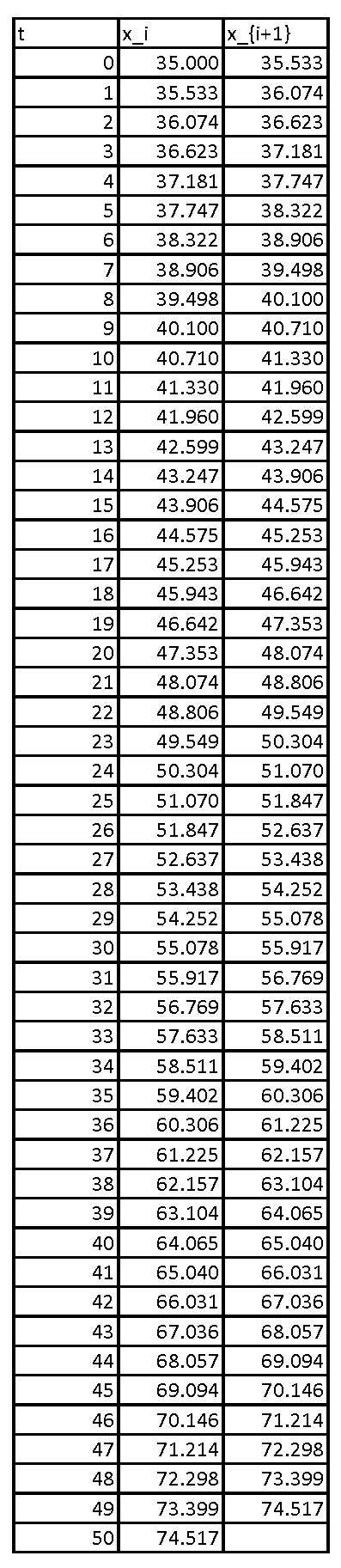
When , the implicit method provides an error similar to that of the explicit method:

When , the IVP is given by:

Given a value for at , and taking , the estimate for can be calculated according to the formula:

Rearranging yields:

With million and years, the estimate for the population at years using the implicit Euler method is given by:

at years, the value of in millions is given by:

Proceeding iteratively, the following is the Excel table showing the values of the population up to years.

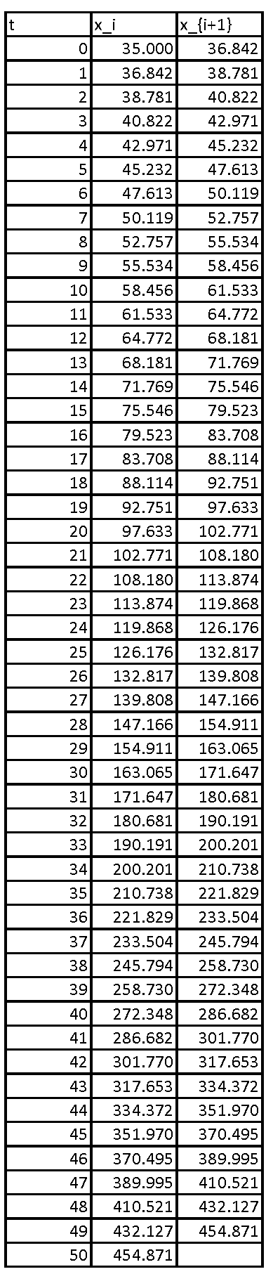
Again, the error produced by the implicit method is comparable to that produced by the explicit method shown above:

The following is the graph showing the exact solution versus the data using both the implicit (blue dots) and the explicit (black dots) Euler method for both values of .

View Mathematica Code

EulerMethod[fp_, x0_, h_, t0_, tmax_] := 
(n = (tmax - t0)/h + 1;
  xtable = Table[0, {i, 1, n}];
  xtable[[1]] = x0;
  Do[xtable[[i]] = xtable[[i - 1]] + h*fp[xtable[[i - 1]], t0 + (i - 2) h], {i, 2, n}];
  Data = Table[{t0 + (i - 1)*h, xtable[[i]]}, {i, 1, n}];
  Data)

ImplicitEulerMethod[fp_, x0_, h_, t0_,  tmax_] := 
(n = (tmax - t0)/h + 1;
  xtable = Table[0, {i, 1, n}];
  xtable[[1]] = x0;
  Do[s = FindRoot[x == xtable[[i - 1]] + h*fp[x, t0 + (i - 1) h], {x, xtable[[i - 1]]}]; xtable[[i]] = x /. s[[1]], {i, 2, n}];
  Data2 = Table[{t0 + (i - 1)*h, xtable[[i]]}, {i, 1, n}];
  Data2)

Clear[x, xtable]
k = 0.015;
a = DSolve[{x'[t] == k*x[t], x[0] == 35}, x, t];
x = x[t] /. a[[1]]
fp[x_, t_] := k*x;
Data = EulerMethod[fp, 35, 1.0, 0, 50];
Data2 = ImplicitEulerMethod[fp, 35, 1.0, 0, 50];
Plot[x, {t, 0, 50}, Epilog -> {PointSize[Large], Point[Data], Blue, Point[Data2]}, AxesOrigin -> {0, 0}, AxesLabel -> {"Time (years)", "Population (Millions)"}]

Clear[x, xtable]
k = 0.05;
a = DSolve[{x'[t] == k*x[t], x[0] == 35}, x, t];
x = x[t] /. a[[1]]
fp[x_, t_] := k*x;
Data = EulerMethod[fp, 35, 1.0, 0, 50];
Data2 = ImplicitEulerMethod[fp, 35, 1.0, 0, 50];
Plot[x, {t, 0, 50}, Epilog -> {PointSize[Large], Point[Data], Blue, Point[Data2]}, AxesOrigin -> {0, 0}, AxesLabel -> {"Time (years)", "Population (Millions)"}]

The following tool illustrates the effect of choosing the step size on the difference between the numerical solution obtained using the implicit methods (shown as dots) and the exact solution (shown as the blue curve) for the case when . The smaller the step size, the more accurate the solution is. The higher the value of , the more the numerical solution deviates from the exact solution. The error increases away from the initial conditions.

Example 2

Repeat Example 2 above using the implicit Euler method.

Solution

Recall that the IVP for this problem is given by:

Taking day, can be predicted for a given value of using the implicit Euler method as follows:

Rearranging:

With and ppb, is calculated as:

Proceeding iteratively produces the following graph with results almost identical to those produced by the explicit method. You can download the Microsoft Excel file example2implicit.xlsx showing the calculations.

ImplicitEulerMethod[fp_, x0_, h_, t0_, tmax_] :=
 (n = (tmax - t0)/h + 1;
  xtable = Table[0, {i, 1, n}];
  xtable[[1]] = x0;
  Do[s = FindRoot[x == xtable[[i - 1]] + h*fp[x, t0 + (i - 1) h], {x, xtable[[i - 1]]}]; xtable[[i]] = x /. s[[1]], {i, 2, n}];
  Data = Table[{t0 + (i - 1)*h, xtable[[i]]}, {i, 1, n}];
  Data)

f[t_] := 100 + 50*Cos[2 Pi*t/365];
cin[t_] := 5 E^(-2 t/1000);
fp[c_, t_] := f[t] (cin[t] - c)/10000;
Data = ImplicitEulerMethod[fp, 5, 1, 0, 365*2];
ListPlot[Data, AxesLabel -> {"time (days)", "Concentration ppb"}]

Example 3

We will repeat Example 3 above to illustrate that the implicit Euler method is always stable.
Consider the IVP of the form:

If , compare the two solutions taking a step size of , and a step size of .

Solution

Using an implicit Euler scheme, the value of can be obtained as follows:

Therefore:

is a positive number. Therefore, the term is bounded for every and therefore, is bounded. The following tool illustrates the difference between the obtained result for . Vary the value of and notice how the obtained solution (black dots) compares to the exact solution (blue curve). While the accuracy is lost with higher values of , the solution maintains numerical stability.

Example 4

Consider the following nonlinear IVP:

with the initial condition . Find the values of for taking using the implicit Euler method.

Solution

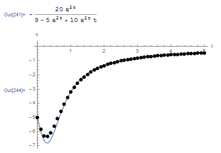
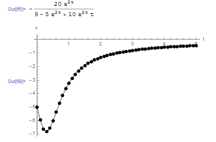
Using Mathematica, the exact solution to the differential equation given can be obtained as:

The implicit Euler scheme provides the following estimate for :

Since appears on both sides, and the equation is nonlinear in , therefore, the Newton-Raphson method will be used at each time increment to find the value of !
Setting , , , and yields:

Solving the above nonlinear equation in using the Newton-Raphson method yields:

Similarly, with , the equation for is:

Using the Newton-Raphson method:

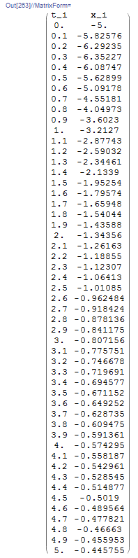
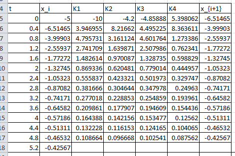
Proceeding iteratively produces the following table:

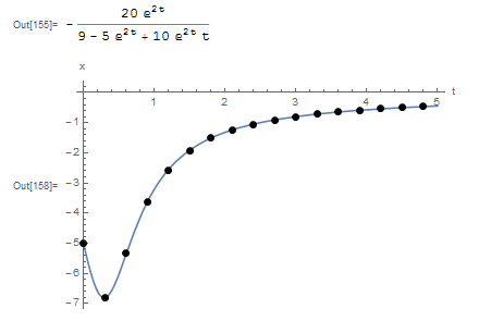
The following is the plot of the exact solution (blue line) with the data obtained using the implicit Euler method. The Mathematica code is given below.

ImplicitEulerMethod[fp_, x0_, h_, t0_, tmax_] := 
(n = (tmax - t0)/h + 1;
  xtable = Table[0, {i, 1, n}];
  xtable[[1]] = x0;
  Do[s = FindRoot[x == xtable[[i - 1]] + h*fp[x, t0 + (i - 1) h], {x, xtable[[i - 1]]}]; xtable[[i]] = x /. s[[1]], {i, 2, n}];
  Data2 = Table[{t0 + (i - 1)*h, xtable[[i]]}, {i, 1, n}];
  Data2)

Clear[x, xtable]
a = DSolve[{x'[t] == t*x[t]^2 + 2*x[t], x[0] == -5}, x, t];
x = x[t] /. a[[1]]
fp[x_, t_] := t*x^2 + 2*x;
Data2 = ImplicitEulerMethod[fp, -5.0, 0.1, 0, 5];
Plot[x, {t, 0, 5}, Epilog -> {PointSize[Large], Point[Data2]},AxesOrigin -> {0, 0}, AxesLabel -> {"t", "x"}, PlotRange -> All]
Title = {"t_i", "x_i"};
Data2 = Prepend[Data2, Title];
Data2 // MatrixForm

Heun’s Method

Heun’s method provides a slight modification to both the implicit and explicit Euler methods. Consider the following IVP:

Assuming that the value of the dependent variable (say ) is known at an initial value , then, we have:

Therefore:

If the trapezoidal rule is used for the right-hand side with one interval we obtain:

where the error term is inherited from the use of the trapezoidal integration rule. Therefore an estimate for is given by:

Using this estimate, the local truncation error is thus proportional to the cube of the step size. If the errors from each interval are added together, with being the number of intervals and the total length , then, the total error is:

which is better than both the implicit and explicit Euler methods. Note that Heun’s method is essentially a slight modification to the Euler’s method in which the slope used to calculate the value of at the next time point is used as the average slope at and at . Heun’s method can be implemented in two ways. One way is to use the slope at to calculate an initial estimate . Then, the estimate for would be calculated based on the slopes at and . Alternatively, the Newton-Raphson method or the fixed-point iteration method can be used to solve directly for . We will only adopt the first way. The following Mathematica code presents a procedure to utilize Heun’s method. The procedure is essentially similar to the ones presented in the Euler methods except for the step to calculate the new estimate .
View Mathematica Code

HeunMethod[fp_, x0_, h_, t0_, tmax_] := 
(n = (tmax - t0)/h + 1;
  xtable = Table[0, {i, 1, n}];
  xtable[[1]] = x0;
  Do[xi0 = xtable[[i - 1]] + h*fp[xtable[[i - 1]], t0 + (i - 2) h]; 
   xtable[[i]] = xtable[[i - 1]] + h (fp[xtable[[i - 1]], t0 + (i - 2) h] +fp[xi0, t0 + (i - 1) h])/2, {i, 2, n}];
  Data = Table[{t0 + (i - 1)*h, xtable[[i]]}, {i, 1, n}];
  Data)

Example

Solve Example 4 above using Heun’s method.

Solution

Heun’s method is implemented by first assuming an estimate for based on the explicit Euler method:

Then, the estimate for is calculated as:

Setting , , , and , an initial estimate for is given by:

Using this information, the slope at can be calculated and used to estimate :

Similarly, an initial estimate for is given by:

Using this information, the slope at can be calculated and used to estimate :

Proceeding iteratively gives the values of up to . The Microsoft Excel file Heun.xlsx provides the required calculations.

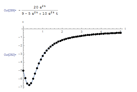
The following graph shows the produced numerical data (black dots) overlapping the exact solution (blue line). The Mathematica code is given below.

HeunMethod[fp_, x0_, h_, t0_, tmax_] := (n = (tmax - t0)/h + 1;
  xtable = Table[0, {i, 1, n}];
  xtable[[1]] = x0;
  Do[xi0 = xtable[[i - 1]] + h*fp[xtable[[i - 1]], t0 + (i - 2) h]; 
   xtable[[i]] =  xtable[[i - 1]] +   h (fp[xtable[[i - 1]], t0 + (i - 2) h] +  fp[xi0, t0 + (i - 1) h])/2, {i, 2, n}];
  Data = Table[{t0 + (i - 1)*h, xtable[[i]]}, {i, 1, n}];
  Data)
Clear[x, xtable]
a = DSolve[{x'[t] == t*x[t]^2 + 2*x[t], x[0] == -5}, x, t];
x = x[t] /. a[[1]]
fp[x_, t_] := t*x^2 + 2*x;
Data2 = HeunMethod[fp, -5.0, 0.1, 0, 5];
Plot[x, {t, 0, 5}, Epilog -> {PointSize[Large], Point[Data2]}, AxesOrigin -> {0, 0}, AxesLabel -> {"t", "x"}, PlotRange -> All]
Title = {"t_i", "x_i"};
Data2 = Prepend[Data2, Title];
Data2 // MatrixForm

The following tool provides a comparison between the explicit Euler method and Heun’s method. Notice that around , the function varies highly in comparison to the rest of the domain. The biggest difference between Heun’s method and the Euler method can be seen when around this area. Heun’s method is able to trace the curve while the Euler method has higher deviations.

The Midpoint Method

Similar to Heun’s method, the midpoint method provides a slight modification to both the implicit and explicit Euler methods. Consider the following IVP:

Assuming that the value of the dependent variable (say ) is known at an initial value , then, we have:

Therefore:

If the midpoint rule of the rectangle method of numerical integration is used for the right-hand side with one interval we obtain:

where the error term is inherited from the use of in the rectangle rule. Therefore an estimate for is given by:

Using this estimate, the local truncation error is thus proportional to the cube of the step size. If the errors from each interval are added together, with being the number of intervals and the total length , then, the total error is:

which is similar to Heun’s method but better than both the implicit and explicit Euler methods. Note that the midpoint method is essentially a slight modification to the Euler’s method in which the slope used to calculate the value of at the next time point is used as the slope at the average point . The midpoint method can be implemented in two ways. One way is to use the slope at to calculate an initial estimate . Then, the estimate for would be calculated based on the slope at . Alternatively, the Newton-Raphson method or the fixed-point iteration method can be used to solve directly for . We will only adopt the first way. The following Mathematica code presents a procedure to utilize the midpoint method. The procedure is essentially similar to the ones presented in the Euler methods except for the step to calculate the new estimate .
View Mathematica Code

MidPointMethod[fp_, x0_, h_, t0_, tmax_] := 
(n = (tmax - t0)/h + 1;
  xtable = Table[0, {i, 1, n}];
  xtable[[1]] = x0;
  Do[xi120 = xtable[[i - 1]] + h/2*fp[xtable[[i - 1]], t0 + (i - 2) h]; 
   xtable[[i]] = xtable[[i - 1]] + h (fp[xi120, t0 + (i - 1-1/2) h]), {i, 2, n}];
  Data = Table[{t0 + (i - 1)*h, xtable[[i]]}, {i, 1, n}];
  Data)

Example

Solve Example 4 above using the midpoint method.

Solution

The midpoint method is implemented by first assuming an estimate for based on the explicit Euler method:

Then, the estimate for is calculated as:

Setting , , , and , an initial estimate for is given by:

Using this information, the slope at can be calculated and used to estimate :

Similarly, an initial estimate for is given by:

Using this information, the slope at can be calculated and used to estimate :

Proceeding iteratively gives the values of up to . The Microsoft Excel file MidPoint.xlsx provides the required calculations.

The following graph shows the produced numerical data (black dots) overlapping the exact solution (blue line). The Mathematica code is given below.

MidPointMethod[fp_, x0_, h_, t0_, tmax_] := (n = (tmax - t0)/h + 1;
  xtable = Table[0, {i, 1, n}];
  xtable[[1]] = x0;
  Do[xi120 = xtable[[i - 1]] + h/2*fp[xtable[[i - 1]], t0 + (i - 2) h];
   xtable[[i]] =  xtable[[i - 1]] + h (fp[xi120, t0 + (i - 1 - 1/2) h]), {i, 2, n}];
  Data2 = Table[{t0 + (i - 1)*h, xtable[[i]]}, {i, 1, n}];
  Data2)
Clear[x, xtable]
a = DSolve[{x'[t] == t*x[t]^2 + 2*x[t], x[0] == -5}, x, t];
x = x[t] /. a[[1]]
fp[x_, t_] := t*x^2 + 2*x;
Data2 = MidPointMethod[fp, -5.0, 0.1, 0, 5];
Plot[x, {t, 0, 5}, Epilog -> {PointSize[Large], Point[Data2]}, AxesOrigin -> {0, 0}, AxesLabel -> {"t", "x"}, PlotRange -> All]
Title = {"t_i", "x_i"};
Data2 = Prepend[Data2, Title];
Data2 // MatrixForm

The following tool provides a comparison between the explicit Euler method and the midpoint method. The midpoint method behaves very similar to Heun’s method. Notice that around , the function varies highly in comparison to the rest of the domain. The biggest difference between midpoint method and the Euler method can be seen when around this area. The midpoint method is able to trace the curve while the Euler method has higher deviations.

Runge-Kutta Methods

The Runge-Kutta methods developed by the German mathematicians C. Runge and M.W. Kutta are essentially a generalization of all the previous methods. Consider the following IVP:

Assuming that the value of the dependent variable (say ) is known at an initial value , then, the Runge-Kutta methods employ the following general equation to calculate the value of at , namely with :

where is a function of the form:

are constants while evaluated at points within the interval and have the form:

The constants , and the forms of are obtained by equating the value of obtained using the Runge-Kutta equation to a particular form of the Taylor series. The are recurrence relationships, meaning appears in , which appears in , and so forth. This makes the method efficient for computer calculations. The error in a particular form depends on how many terms are used. The general forms of these Runge-Kutta methods could be implicit or explicit. For example, the explicit Euler method is a Runge-Kutta method with only one term with and . Heun’s method on the other hand is a Runge-Kutta method with the following non-zero terms:

Similarly, the midpoint method is a Runge-Kutta method with the following non-zero terms:

The most popular Runge-Kutta method is referred to as the “classical Runge-Kutta method”, or the “fourth-order Runge-Kutta method”. It has the following form:

with

The error in the fourth-order Runge-Kutta method is similar to that of the Simpson’s 1/3 rule, with a local error term which would translate into a global error term of . The method is termed fourth-order because the error term is directly proportional to the step size raised to the power of 4.

RK4Method[fp_, x0_, h_, t0_, tmax_] := (n = (tmax - t0)/h + 1;
  xtable = Table[0, {i, 1, n}];
  xtable[[1]] = x0;
  Do[k1 = fp[xtable[[i - 1]], t0 + (i - 2) h];
   k2 = fp[xtable[[i - 1]] + h/2*k1, t0 + (i - 1.5) h];
   k3 = fp[xtable[[i - 1]] + h/2*k2, t0 + (i - 1.5) h];
   k4 = fp[xtable[[i - 1]] + h*k3, t0 + (i - 1) h];
   xtable[[i]] = xtable[[i - 1]] + h (k1 + 2 k2 + 2 k3 + k4)/6, {i, 2,
     n}];
  Data2 = Table[{t0 + (i - 1)*h, xtable[[i]]}, {i, 1, n}];
  Data2)

Example

Solve Example 4 above using the classical Runge-Kutta method but with .

Solution

Recall the differential equation of this problem:

Setting , , , the following are the values of , , , and required to calculate :

Therefore:

Proceeding iteratively gives the values of up to . The Microsoft Excel file RK4.xlsx provides the required calculations. The following Microsoft Excel table shows the required calculations:

The following Mathematica code implements the classical Runge-Kutta method for this problem with . The output curve is shown underneath.
View Mathematica Code

RK4Method[fp_, x0_, h_, t0_, tmax_] := (n = (tmax - t0)/h + 1;
  xtable = Table[0, {i, 1, n}];
  xtable[[1]] = x0;
  Do[k1 = fp[xtable[[i - 1]], t0 + (i - 2) h];
   k2 = fp[xtable[[i - 1]] + h/2*k1, t0 + (i - 1.5) h];
   k3 = fp[xtable[[i - 1]] + h/2*k2, t0 + (i - 1.5) h];
   k4 = fp[xtable[[i - 1]] + h*k3, t0 + (i - 1) h];
   xtable[[i]] = xtable[[i - 1]] + h (k1 + 2 k2 + 2 k3 + k4)/6, {i, 2,
     n}];
  Data2 = Table[{t0 + (i - 1)*h, xtable[[i]]}, {i, 1, n}];
  Data2)
Clear[x, xtable]
a = DSolve[{x'[t] == t*x[t]^2 + 2*x[t], x[0] == -5}, x, t];
x = x[t] /. a[[1]]
fp[x_, t_] := t*x^2 + 2*x;
Data2 = RK4Method[fp, -5.0, 0.3, 0, 5];
Plot[x, {t, 0, 5}, Epilog -> {PointSize[Large], Point[Data2]},  AxesOrigin -> {0, 0}, AxesLabel -> {"t", "x"}, PlotRange -> All]
Title = {"t_i", "x_i"};
Data2 = Prepend[Data2, Title];
Data2 // MatrixForm

The following tool provides a comparison between the explicit Euler method and the classical Runge-Kutta method. The classical Runge-Kutta method gives excellent predictions even when , at which point the explicit Euler method fails to predict anything close to the exact equation. The classical Runge-Kutta method also provides better estimates than the midpoint method and Heun’s method above.

Solving Systems of IVPs

Many engineering problems contain systems of IVPs in which more than one dependent variable is a function of one independent variable, say . For example, chemical reactions of more than one component are usually described using systems of IVPs in which the initial conditions are known. Similarly, the interaction of biological growth of different species (predators and prey) is usually represented by a system of IVPs in which the initial conditions are given. Generally, these systems can be represented as:

The independent variable is discretized such that with a constant step . In such systems, the initial conditions, namely the values of , are given. The values of when are denoted: . In this case, the values of the dependent variables at can be obtained using the following system of equations:

where depend on the method used. For example, if the explicit Euler method is used, then:

Alternatively, if the classical Runge-Kutta method is used, then:

where , , , and are the values associated with the dependent variable and calculated according to the classical Runge-Kutta technique.

It should also be noted that higher-order IVPs can be solved by converting them into a system of first-order IVPs. For example, consider the IVP:

with the initial conditions and given. Then, setting , the equation can be written as a system of two IVPs:

with initial conditions given for and .

Example

Consider the damped mechanical system with , , with the initial conditions . Find the numerical solution for the position and the velocity for using the explicit Euler method and the Runge-Kutta method. Use .

Solution

The differential equation of the damped system is given by:

The following exact solution can be obtained using the built-in DSolve function in Mathematica:

To find the numerical solution, the equation will be converted into a system of 2 IVPs. Setting , the equation can be converted into the following system:

with the initial conditions . With , the interval can be split into time steps. The time discretization will be such that , , , up to . The corresponding positions are given by: while the corresponding velocities are given by: .

Explicit Euler Method

Using the explicit Euler method, the values of and can be evaluated as:

With the initial conditions , the values of and at can be calculated as:

Similarly, the values of and can be obtained as:

Proceeding iteratively, the values of and up to can be obtained. The Microsoft Excel file EulerSystem.xlsx shows the obtained values.

Classical Runge-Kutta method

The two differential equations are designated and as follows:

Using the classical Runge-Kutta method, the values of and can be evaluated as:

where:

With the initial conditions , the values of can be calculated as:

Therefore:

For and , the values of can be calculated as:

Therefore:

Proceeding iteratively, the values of and up to can be obtained. The Microsoft Excel file RK4System.xlsx shows the calculated up to the required time point.

Comparison

The following figure shows the exact solution (blue curve) and the numerical solution (black dots) for the position and the velocity obtained using the explicit Euler method and the classical Runge-Kutta method. Using the explicit Euler method, the numerical solution deviates from the exact solution for higher values of . However, the classical Runge-Kutta method provides very accurate predictions. The Mathematica code utilized to produce the curves is shown below.

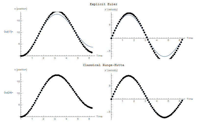
Clear[x]
a = DSolve[{x''[t] == 10 - x[t] - 0.15 x'[t], x'[0] == 0, x[0] == 0}, x, t]
x = x[t] /. a[[1]]
xp = Simplify[D[x, t]]

Plot[x, {t, 0, 2 Pi}, AxesOrigin -> {0, 0}, AxesOrigin -> {0, 0}, AxesLabel -> {"time", "x (position)"}]
Plot[xp, {t, 0, 2 Pi}, AxesOrigin -> {0, 0}, AxesOrigin -> {0, 0}, AxesLabel -> {"time", "x' (velocity)"}]

EulerMethod2[fp1_, fp2_, x10_, x20_, h_, t0_, tmax_] := (
  n = (tmax - t0)/h + 1;
  x1table = Table[0, {i, 1, n}];
  x2table = Table[0, {i, 1, n}];
  x1table[[1]] = x10;
  x2table[[1]] = x20;
  Do[x1table[[i]] = x1table[[i - 1]] +   h*fp1[x1table[[i - 1]], x2table[[i - 1]], t0 + (i - 2) h];
   x2table[[i]] = x2table[[i - 1]] +  h*fp2[x1table[[i - 1]], x2table[[i - 1]], t0 + (i - 2) h], 
    {i, 2,     n}];
  Data = Table[{t0 + (i - 1)*h, x1table[[i]], x2table[[i]]}, {i, 1,  n}];
  Data)

RK4Method2[fp1_, fp2_, x10_, x20_, h_, t0_,   tmax_] := (
  n = (tmax - t0)/h + 1;
  x1table = Table[0, {i, 1, n}];
  x1table[[1]] = x10;
  x2table = Table[0, {i, 1, n}];
  x2table[[1]] = x20;
  Do[k11 = fp1[x1table[[i - 1]], x2table[[i - 1]], t0 + (i - 2) h];
   k21 = fp2[x1table[[i - 1]], x2table[[i - 1]], t0 + (i - 2) h];
   k12 = fp1[x1table[[i - 1]] + h/2*k11, x2table[[i - 1]] + h/2*k21,      t0 + (i - 1.5) h];
   k22 = fp2[x1table[[i - 1]] + h/2*k11, x2table[[i - 1]] + h/2*k21,      t0 + (i - 1.5) h];
   k13 = fp1[x1table[[i - 1]] + h/2*k12, x2table[[i - 1]] + h/2*k22,      t0 + (i - 1.5) h];
   k23 = fp2[x1table[[i - 1]] + h/2*k12, x2table[[i - 1]] + h/2*k22,      t0 + (i - 1.5) h];
   k14 = fp1[x1table[[i - 1]] + h*k13, x2table[[i - 1]] + h*k23,      t0 + (i - 1) h];
   k24 = fp2[x1table[[i - 1]] + h*k13, x2table[[i - 1]] + h*k23,      t0 + (i - 1) h];
   x1table[[i]] = x1table[[i - 1]] + h (k11 + 2 k12 + 2 k13 + k14)/6;
   x2table[[i]] = x2table[[i - 1]] + h (k21 + 2 k22 + 2 k23 + k24)/6, {i, 2, n}];
  Data2 = Table[{t0 + (i - 1)*h, x1table[[i]], x2table[[i]]}, {i, 1, n}];
  Data2)


fp1[x_, y_, t_] := y;
fp2[x_, y_, t_] := 10 - x - 0.15 y;
Data = EulerMethod2[fp1, fp2, 0, 0, 0.1, 0, 2 Pi];
DataPosition = Drop[Data, None, {3}];
DataVelocity = Drop[Data, None, {2}];
a1 = Plot[x, {t, 0, 6.3},   Epilog -> {PointSize[Large], Point[DataPosition]},    AxesOrigin -> {0, 0}, ImageSize -> Medium,    AxesLabel -> {"Time", "x (position)"}];
a2 = Plot[xp, {t, 0, 6.3},    Epilog -> {PointSize[Large], Point[DataVelocity]},    AxesOrigin -> {0, 0}, ImageSize -> Medium,    AxesLabel -> {"Time", "x' (velocity)"}];
a = Grid[{{a1, a2}}];
Grid[{{"Explicit Euler"}, {a}}]
Data = RK4Method2[fp1, fp2, 0, 0, 0.1, 0, 2 Pi];
DataPosition = Drop[Data, None, {3}];
DataVelocity = Drop[Data, None, {2}];
a1 = Plot[x, {t, 0, 6.3},    Epilog -> {PointSize[Large], Point[DataPosition]},    ImageSize -> Medium, AxesOrigin -> {0, 0},    AxesLabel -> {"Time", "x (position)"}];
a2 = Plot[xp, {t, 0, 6.3},    Epilog -> {PointSize[Large], Point[DataVelocity]},    ImageSize -> Medium, AxesOrigin -> {0, 0},    AxesLabel -> {"Time", "x' (velocity)"}];
a = Grid[{{a1, a2}}];
Grid[{{"Classical Runge-Kutta"}, {a}}]

The effect of changing the value of on the resulting numerical solution for the system of IVPs given here can be illustrated using the following tool. Even for the classical Runge-Kutta produces very accurate predictions at which point the explicit Euler method produces very erroneous results.

Using Mathematica

The built-in NDSolve in Mathematica uses the Runge-Kutta methods to solve a system of IVPs and produces piecewise interpolating polynomials for the dependent variables. The following code solves some of the preceding examples and compares with the exact solution. Note that in those examples when the exact and numerical solutions are plotted together, they overlap!

Clear[x, xn, xtable]
(*Example 1*)
k = 0.015;
a = DSolve[{x'[t] == k*x[t], x[0] == 35}, x, t];
x = x[t] /. a[[1]]

b = NDSolve[{xn'[t] == k*xn[t], xn[0] == 35}, xn, {t, 0, 50}]
xn = xn /. b[[1]]
Plot[{x, xn[t]}, {t, 0, 50}, PlotLegends -> {"Exact", "Numerical using Mathematica"}, AxesLabel -> {"t", "Population"}]

(*Example 2*)
Clear[cn]
b = NDSolve[{cn'[t] == (100 + 50*Cos[2 Pi*t/365])/10000*(5 Exp[-2 t/1000] - cn[t]), cn[0] == 5}, cn, {t, 0, 700}]
cn = cn /. b[[1]]
Plot[cn[t], {t, 0, 700}, AxesLabel -> {"t", "Concentration"}]


(*Example 4*)

Clear[xn, x]
a = DSolve[{x'[t] == t*x[t]^2 + 2*x[t], x[0] == -5}, x, t];
x = x[t] /. a[[1]]
b = NDSolve[{xn'[t] == t*xn[t]^2 + 2 xn[t], xn[0] == -5},  xn, {t, 0, 5}]
xn = xn /. b[[1]]
Plot[{x, xn[t]}, {t, 0, 5}, PlotRange -> All, PlotLegends -> {"Exact", "Numerical using Mathematica"}, AxesLabel -> {"t", "x"}]

(*Example of a system*)
Clear[xn, yn, x]
a = DSolve[{x''[t] == 10 - x[t] - 0.15 x'[t], x'[0] == 0, x[0] == 0},   x, t]
x = x[t] /. a[[1]]
xp = Simplify[D[x, t]]
b = NDSolve[{xn'[t] == yn[t], yn'[t] == 10 - xn[t] - 0.15 yn[t],    xn[0] == 0, yn[0] == 0}, {xn, yn}, {t, 0, 2 Pi}]
xn = xn /. b[[1]]
yn = yn /. b[[1]]

Plot[{x, xn[t]}, {t, 0, 2 Pi}, AxesOrigin -> {0, 0},  AxesOrigin -> {0, 0},  PlotLegends -> {"Exact", "Numerical using Mathematica"},  AxesLabel -> {"time", "x (position)"}]
Plot[{xp, yn[t]}, {t, 0, 2 Pi}, AxesOrigin -> {0, 0},  AxesOrigin -> {0, 0},  PlotLegends -> {"Exact", "Numerical using Mathematica"},  AxesLabel -> {"time", "x' (velocity)"}]

Solution Methods for BVPs

As mentioned above, BVP are ordinary differential equations whose boundary conditions are given at different values of the independent variable. Usually, these points are the extreme points of the region of interest, or the “boundaries” of the domain and hence the term: “boundary value problem”. Consider a BVP with as the dependent variable and as the independent variable. The boundary conditions would be given in terms of or the derivatives of at different values of the independent variable . When the boundary conditions are given in terms of , then, this type of boundary conditions is termed Dirichlet boundary condition. Otherwise, when the boundary conditions are given in terms of the derivatives of , this type of boundary conditions is termed Neumann boundary condition. A BVP is usually an ODE that is at least of the second-order as equations of the first order require only one boundary condition which is usually an initial boundary condition. There are various methods to solve boundary value problems; among them are the following:

1. Shooting method. In the shooting method the boundary value problem is solved as an initial value problem and the initial conditions are varied until the boundary conditions at the extreme ends are satisfied. For example, consider the BVP

      

   with the boundary conditions:

      

   Then, the system can be converted into an initial value problem with the following boundary conditions:

      

   After a solution is obtained, the value of is compared to and is varied and the solution is repeated until .

2. Finite difference method. The finite difference method relies on approximating the BVP with difference equations by replacing the derivatives of the function with their finite difference approximations.
3. Weak formulation methods. The weak formulation methods rely on converting the problem into a different “integral” form and finding the best solution that would satisfy the new form. Examples of such methods are the finite element analysis method or the weighted residuals methods.

The finite difference method is the only method that we will cover in these notes.

Finite Difference Method

Consider a BVP with the dependent variable and the independent variable with . The finite difference method in a BVP relies on discretizing the domain into intervals with with a constant step size . The values of the dependent variable at the interval junctions are denoted by: . The finite difference method seeks to find a numerical solution to each by solving difference equations formed by replacing the derivatives in the BVP with a finite difference approximation scheme (usually the centred finite difference scheme). Dirichlet boundary conditions can be directly imposed on the known values of while Neumann boundary conditions can be imposed as additional difference equations using an appropriate finite difference scheme. The following examples show how the method can be implemented.

Example 1

In this example, we first derive the heat equation and then attempt to solve it using the finite difference method.
Heat Equation Derivation: The differential equation describing thermal energy within objects (Steady State Heat Equation) is one example of a BVP that can be solved using the finite difference method. In this example, the steady state heat equation is first derived for a one-dimensional rod of length 10m connecting two heat sources of constant temperature as shown in the figure such that the temperature of the rod at the end is equal to C while the temperature at the other end is equal to C. The ambient temperature around the rod is equal to C. The steady state heat equation can be derived by balancing the amount of heat energy per unit time entering and exiting through a control length of the rod. The amount of heat energy transferred to the ambient environment per unit time and per unit length is equal to

With units for this example. The amount of heat energy transferred through the rod per unit time is equal to:

With units in this example. The negative sign is essential as heat energy is transferred from areas of high temperature to areas of lower temperature. The steady state differential equation can be derived by equating the amount of energy entering to the amount of energy exiting per unit time considering a control length equal to as shown in the figure below:

Where a Taylor series with only two terms was used to approximate . Therefore:

The solution to this equation provides the temperature distribution (with being the dependent variable) within the rod (with as the independent variable).

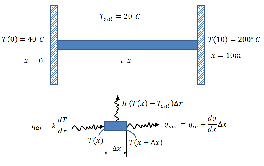
Statement of Problem: Consider the BVP developed above with the Dirichlet boundary conditions and .

1. Find the exact solution of the differential equation.
2. Use the finite difference method with intervals to find a numerical solution to the BVP.

Repeat the problem considering the two boundary conditions: the Dirichlet boundary condition and the Neumann boundary condition

Solution

Dirichlet Boundary Conditions
The exact solution can be directly obtained in Mathematica using the DSolve function. Note that an exact solution is not always available.

The numerical solution is obtained by first discretizing the domain into intervals with and . The values of at these points are denoted by . The boundary conditions are given as Dirichlet type with and . The remaining 3 unknowns can be obtained by utilizing the basic formulas of the centred finite difference scheme to replace the derivatives in the differential equation. These can be utilized to write 4 equations of the form:

This results in the following three equations (after the substitution and ):

Rearranging yields the following linear system of equations:

Solving the above system yields:

Combined with and , a list plot can be drawn to show the obtained numerical solution. The following figure shows the exact solution (blue curve) with the numerical solution (black dots). The figure shows that the numerical solution is almost identical to the exact solution.

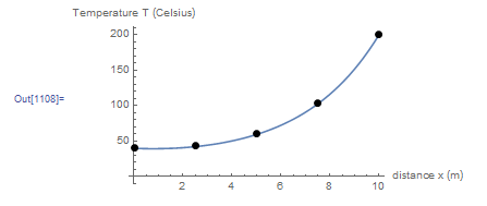
View Mathematica Code

ClearAll["Global`*"]
hp = 1/10;
n = 4;
L = 10 - 0;
h = L/n;
Ts = Table[Symbol["T" <> ToString[i]], {i, 0, n}]
T0 = 40;
Ts[[n + 1]] = 200;
Ts // MatrixForm
Equations =   Table[(Ts[[i + 1]] - 2 Ts[[i]] + Ts[[i - 1]])/h^2 ==     hp*(Ts[[i]] - 20), {i, 2, n}];
Equations // MatrixForm
Equations = Expand[Equations];
Equations // MatrixForm
N[Equations] // MatrixForm

unknowns = Table[Symbol["T" <> ToString[i]], {i, 1, n - 1}]
a = Solve[Equations, unknowns]
Ts = Ts /. a[[1]]
SolList = Table[{0 + (i)*h, Ts[[i + 1]]}, {i, 0, n}];
SolList // MatrixForm

a = DSolve[{T''[x] == hp*(T[x] - 20), T[0] == 40, T[10] == 200}, T, x]
T = T[x] /. a[[1]];
FullSimplify[N[T]]
Plot[T, {x, 0, 10},  AxesLabel -> {"distance x (m)", "Temperature T (Celsius)"},  AxesOrigin -> {0, 0}, Epilog -> {PointSize[Large], Point[SolList]}]

In the following tool, vary the number of intervals to show the effect on the numerical solution:

Dirichlet and Neumann Boundary Conditions
The exact solution can be directly obtained in Mathematica using the DSolve function. Note that an exact solution is not always available.

The numerical solution is obtained by first discretizing the domain into intervals with and . The values of at these points are denoted by . The Dirichlet boundary condition can be used to set . The remaining 4 unknowns can be obtained using four equations. Three equations are composed by utilizing the basic formulas of the centred finite difference scheme to replace the derivatives in the differential equation at the three intermediate points. The fourth equation is composed by utilizing the backward finite difference scheme at and equate it to the Neumann boundary condition. The three difference equations at the intermediate points have the form:

This results in the following three equations (after the substitution ):

The fourth equation can be obtained using the backward finite difference at point :

Combining the four equations and rearranging yields the following linear system of equations:

Solving the above system yields:

Combined with , a list plot can be drawn to show the obtained numerical solution. The following figure shows the exact solution (blue curve) with the numerical solution (black dots). The figure shows that the numerical solution of the same differential equation with Neumann boundary conditions provides less accurate results than the solution when Dirichlet boundary conditions were used.

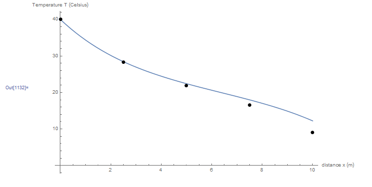
View Mathematica Code

ClearAll["Global`*"]
hp = 1/10;
n = 4;
L = 10 - 0;
h = L/n;
Ts = Table[Symbol["T" <> ToString[i]], {i, 0, n}]
T0 = 40;
Ts // MatrixForm
Equations =   Table[(Ts[[i + 1]] - 2 Ts[[i]] + Ts[[i - 1]])/h^2 ==     hp*(Ts[[i]] - 20), {i, 2, n}];
NeumannEquation = ((Ts[[n + 1]] - Ts[[n]])/h == -3);
Equations = Append[Equations, NeumannEquation];
Equations // MatrixForm
Equations = Expand[Equations];
Equations // MatrixForm
N[Equations] // MatrixForm

unknowns = Table[Symbol["T" <> ToString[i]], {i, 1, n}]
a = Solve[Equations, unknowns];
Ts = N[Ts /. a[[1]]]
SolList = Table[{0 + (i)*h, Ts[[i + 1]]}, {i, 0, n}];
SolList // MatrixForm

a = DSolve[{T''[x] == hp*(T[x] - 20), T[0] == 40, T'[10] == -3}, T, x]
T = T[x] /. a[[1]];
FullSimplify[N[T]]
Plot[T, {x, 0, 10},  AxesLabel -> {"distance x (m)", "Temperature T (Celsius)"},  AxesOrigin -> {0, 0}, Epilog -> {PointSize[Large], Point[SolList]}]

The numerical solution approaches the exact solution as the number of intervals is increased. Vary in the following tool and observe how it affects the numerical solution.

Example 2

Consider the following second-order BVP:

with the boundary conditions:

Use the finite difference method to find a numerical solution to the above equation by dividing the domain into intervals. Compare with the exact solution.

Solution

The exact solution can be directly obtained in Mathematica using the DSolve function. Note that an exact solution is not always available.

The numerical solution is obtained by first discretizing the domain into intervals with and . The values of at these points are denoted by . The boundary conditions are given as Dirichlet type with and . The remaining 4 unknowns can be obtained by utilizing the basic formulas of the centred finite difference scheme to replace the derivatives in the differential equation. These can be utilized to write 4 equations of the form:

This results in the following four equations (after the substitution and ):

Rearranging yields the following linear system of equations:

Solving the above system yields:

Combined with and , a list plot can be drawn to show the obtained numerical solution. The following figure shows the exact solution (blue curve) with the numerical solution (black dots). The maximum error in the numerical solution is obtained at . At this location, the exact solution is given by while the numerical solution is given by with a relative error of -19%:

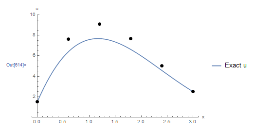
ClearAll["Global`*"]
n = 5;
L = 3 - 0;
h = L/n;
us = Table[Symbol["u" <> ToString[i]], {i, 0, n}]
u0 = 1.5;
us[[n + 1]] = 2.5;
us // MatrixForm
Equations = Table[(us[[i + 1]] - 2 us[[i]] + us[[i - 1]])/h^2 + (us[[i + 1]] - us[[i - 1]])/2/h + us[[i]] == 1, {i, 2, n}];
Equations // MatrixForm
Equations = Expand[Equations];
Equations // MatrixForm
N[Equations] // MatrixForm

unknowns = Table[Symbol["u" <> ToString[i]], {i, 1, n - 1}]
a = Solve[Equations, unknowns]
us = us /. a[[1]]
SolList = Table[{0 + (i)*h, us[[i + 1]]}, {i, 0, n}];
SolList // MatrixForm;

Clear[u]
(*Exact Solution*)
b = DSolve[{u''[x] + u'[x] + u[x] == 1, u[0] == 15/10, u[3] == 25/10},   u, x]
u = FullSimplify[u[x] /. b[[1]], Reals]
Plot[u, {x, 0, 3}, PlotLegends -> {"Exact u"},  AxesLabel -> {"x", "u"},  Epilog -> {PointSize[Large], Point[SolList]},  PlotRange -> {{-0.1, 3.1}, {0, 10}}]
Print["u at x=1.2 is ", uexact = u /. x -> 1.2]
Print["u_2 is ", u2 = u2 /. a[[1]]]
Print["Relative Error is ", (uexact - u2)/uexact]

In a BVP, the accuracy of the solution depends on the accuracy of the finite difference scheme used. As shown in the following tool, by decreasing the value of , the numerical solution gets closer to the exact solution.

Example 3

The differential equation describing the displacement of a hanging chain as a function of the weight per unit length of the chain and the desired horizontal tension in the chain is given by:

Where is the dependent variable being the chain curve and is the independent variable being the horizontal distance. The solution to this equation, namely the function is called the catenary or the curve that describes the hanging chain. See this page for a detailed derivation and some of the properties of the curve.
If the boundary conditions are given by and and if and units, then use the finite difference method to find a numerical solution by dividing the domain into intervals. Compare with the exact solution.

Solution

Notice that this equation is a nonlinear second-order differential equation. Its exact solution describing the catenary of the chain can be obtained using the built-in Integrate function in Mathematica and has the form:

The numerical solution is obtained by first discretizing the domain into intervals with and . The values of at these points are denoted by . The boundary conditions are given as Dirichlet type with and . The remaining 4 unknowns can be obtained by utilizing the basic formulas of the centred finite difference scheme to replace the derivatives in the differential equation. These can be utilized to write 4 nonlinear equations of the form:

This results in the following four nonlinear equations (after the substitution and ):

Notice that the resulting equations are nonlinear because the differential equation itself was nonlinear. The above system can be solved using the Newton-Raphson method with initial guesses of for all of the unknowns which yields the following solution:

Combined with and , a list plot can be drawn to show the obtained numerical solution. The following figure shows the exact solution (blue curve) with the numerical solution (black dots). The two solutions are very close to each other.

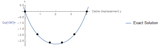
ClearAll["Global`*"]
w = 1.;
T = 1;
a = DSolve[{y''[x] == w/T*Sqrt[1 + (y'[x])^2], y[0] == 0, y[4] == 0},y, x]
y = FullSimplify[y[x] /. a[[1]]]
Plot[y, {x, 0, 4}]
L = 4 - 0
n = 5;
h = L/n;
ys = Table[Symbol["y" <> ToString[i]], {i, 0, n}];
y0 = 0;
ys[[n + 1]] = 0;
ys // MatrixForm
Equations =   Table[(ys[[i + 1]] - 2 ys[[i]] + ys[[i - 1]])/h^2 ==     w/T*Sqrt[1 + ((ys[[i + 1]] - ys[[i - 1]])/2/h)^2], {i, 2, n}];
Equations // MatrixForm
unknowns = Table[Symbol["y" <> ToString[i]], {i, 1, n - 1}];
Initvalues = Table[{unknowns[[i]], -0.1}, {i, 1, n - 1}];
a = FindRoot[Equations, Initvalues]
ys = ys /. a
SolList = Table[{0 + (i)*h, ys[[i + 1]]}, {i, 0, n}];
Plot[y, {x, -0.1, 4.1}, AxesLabel -> {"Cable displacement y", "x"}, PlotLegends -> {"Exact Solution"},  Epilog -> {PointSize[Large], Point[SolList]}]

As shown in the following tool, by decreasing the value of , the numerical solution gets closer to the exact solution.

Example 4

Consider the following BVP

With the boundary conditions and . Assuming , use the finite difference method to find a numerical solution to the given BVP. Compare with the exact solution.

Solution

The exact solution can be directly obtained in Mathematica using the DSolve function.

The numerical solution is obtained by first discretizing the domain into intervals with and , . The values of at these points are denoted by . The boundary conditions are given as Dirichlet type with and . The remaining 9 unknowns can be obtained by utilizing the basic formulas of the centred finite difference scheme to replace the derivatives in the differential equation. These can be utilized to write 9 equations of the form:

This results in the following four equations (after the substitution and ):

Rearranging yields the following linear system of equations:

Solving the above system yields:

Combined with and , a list plot can be drawn to show the obtained numerical solution. The following figure shows the exact solution (blue curve) with the numerical solution (black dots). The numerical solution exactly overlaps the exact solution!

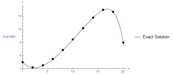
View Mathematica Code

ClearAll["Global`*"]
a = DSolve[{7 y''[x] - 2 y'[x] - y[x] + x == 0, y[0] == 5, y[20] == 8}, y, x]
y = FullSimplify[y[x] /. a[[1]]]
y = FullSimplify[N[y]]
Plot[y, {x, 0, 20}]
L = 20 - 0
n = 10;
h = L/n;
ys = Table[Symbol["y" <> ToString[i]], {i, 0, n}];
y0 = 5;
ys[[n + 1]] = 8;
ys // MatrixForm
Equations =   Table[7 (ys[[i + 1]] - 2 ys[[i]] + ys[[i - 1]])/h^2 -      2 (ys[[i + 1]] - ys[[i - 1]])/2/h - ys[[i]] + 0 + (i - 1)*h ==     0, {i, 2, n}];
Equations // MatrixForm
Expand[N[Equations]] // MatrixForm
unknowns = Table[Symbol["y" <> ToString[i]], {i, 1, n - 1}];
a = Solve[Equations, unknowns];
ys = N[ys /. a[[1]]]
SolList = Table[{0 + (i)*h, ys[[i + 1]]}, {i, 0, n}];
Plot[y, {x, -0.1, 20.1}, AxesLabel -> {"x", "y"},  PlotLegends -> {"Exact Solution"},  Epilog -> {PointSize[Large], Point[SolList]}]

Problems

1. The current code given in the explicit Euler method assumes that is chosen such that is a natural number. Modify the code so that if this is not the case, the solution for the dependent variable at is available.
2. Consider the following IVP:

      

   with the initial condition .

   • Use the built-in DSolve function to find the exact solution and plot for .
   • Use the explicit Euler method with to find the values of . Plot the exact solution overlapping the obtained numerical solution.
   • Use the implicit Euler method with to find the values of . Plot the exact solution overlapping the obtained numerical solution.
   • Use Heun’s method with to find the values of . Plot the exact solution overlapping the obtained numerical solution.
   • Use the midpoint method with to find the values of . Plot the exact solution overlapping the obtained numerical solution.
   • Use the classical Runge-Kutta method with to find the values of . Plot the exact solution overlapping the obtained numerical solution.
3. Consider a mass-spring system with units, units with the initial conditions .
   • Use the built-in DSolve function to find the exact solution and plot the position and velocity for .
   • Use the explicit Euler method with to find the values of and . Plot the exact solutions overlapping the obtained numerical solutions.
   • Use the classical Runge-Kutta method with to find the values of and . Plot the exact solution overlapping the obtained numerical solution.
4. Consider the following IVP:

      

   with the initial conditions and . Use the implicit Euler method to find a numerical solution to the given IVP for with . Compare with the exact solution.

5. Consider the following IVP:

      

   with the initial conditions and . Use the classical 4th-order Runge-Kutta method to find a numerical solution to the given IVP for with . Compare with the exact solution.

6. Consider the following nonlinear system of IVPs:

      

   with the initial conditions , , and . Use the classical 4th-order Runge-Kutta method to find a numerical solution to the given IVP for with . Then, using list plots, plot the three curves showing versus , versus , and versus .
   Note: The above system is an example of a Lorenz system of equations which can have chaotic solutions depending on the parameters used and the initial conditions.

7. Use the finite difference method to find a numerical solution to the following BVP:

      

   with the boundary conditions and . Use intervals, and compare with the exact solution.

8. The deflection as a function of the position along the length of a simply supported Euler-Bernoulli beam uniformly loaded is given by:

      

   Where MPa is the Young’s modulus, is the moment of inertia, is the uniformly distributed load, and m is the length of the beam. The boundary conditions are given by . Use the finite difference method to find a numerical solution to the deflection using intervals. Compare with the exact solution.