Biomechanics and Bioengineering of Orthopaedics: Compression as a failure Mode
This section briefly introduces the buckling phenomenon and mechanical behaviour of bone under compression.
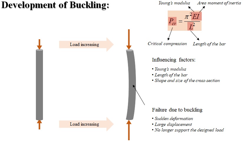
If a structure is subjected to a gradually increasing compressive load, when the load reaches a critical level, the structure suddenly changes shape. This phenomenon is called buckling.
When buckling happens, an initial straight member will deform suddenly, producing large displacements (Fig. 3-1). This doesn’t always cause yielding or fracture of the material, but buckling is a failure mode which indicates that the structure cannot support the designed load any longer. Basically, the critical compression load can be calculated using this Euler’ formula. There are three factors influencing the critical compression load which include the Young’s modulus of the material, length of the bar, and the shape and size of the bar cross-section.
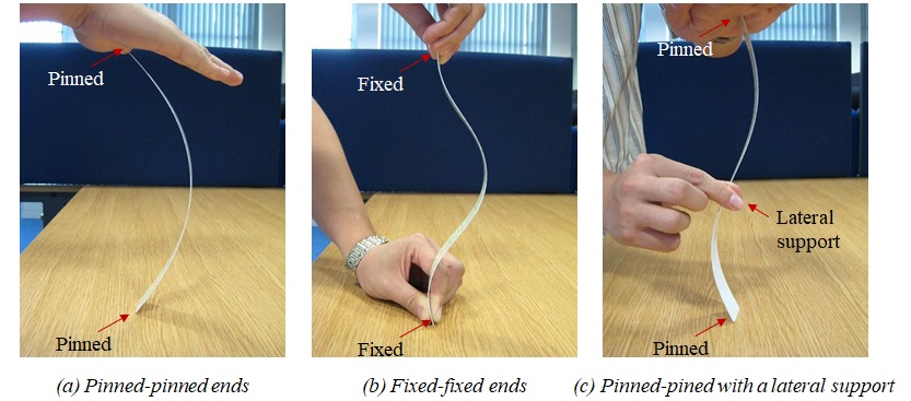
Let’s see a common example of buckling in life. If you have a ruler at hand, you can also conduct the small experiment (Fig. 3-2).
First, put one end of the ruler on the surface of a table and the other end in the palm of one’s hand. The two ends of the ruler are free to rotate at their locations. This kind of condition applied to the end is called pin, which means the end of ruler is pinned. Now, press axially on the top end of the ruler and gradually increase the compression force. The straight ruler will suddenly deflect laterally as shown in the figure. Remember your feeling of the force that you applied on the ruler. If you increase force, the deformation becomes larger. This simulates the buckling of a column with two pinned ends.
Now, let’s hold the two ends of the ruler tightly to prevent any rotational and lateral movements of the two ends of the ruler. The ruler ends are fixed at that location, and rotation is not allowed. This is called fixed-end condition. Then gradually press axially on the ruler using the fingers until the ruler deforms sideways as shown in the figure. In this case, you will see a different buckling shape from the first one. Also, remember the feel of your hands and compare it with your applied force in the last experiment. You can clearly feel that a larger force is needed in this demonstration than in the previous demonstration!
Let’s go back to the first experiment, the pined-to-pined ends conditions. But this time, we apply a lateral support which just restrain that section at that location but allow the section to rotate. Press axially on the top end of the ruler and gradually increase the compression force. You can feel that a larger compressive force will be required to make the ruler buckle in the shape shown in the figure.
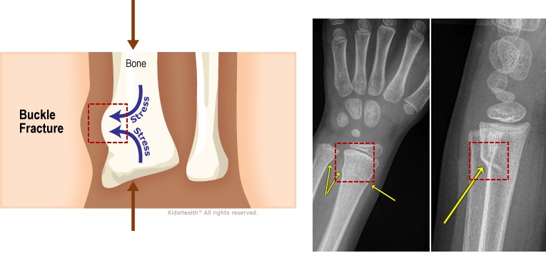
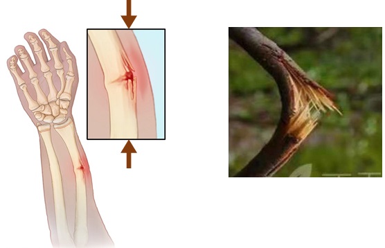
A failure mode of bone could be due to buckling. This failure mode is called buckle fracture, which is also referred to as impact fracture. In this fracture, one side of a bone bends, raising a buckle, without breaking the other side of the bone (Fig. 3-3). It usually happens when sudden compression is applied to bone.
This type of fracture usually happens in children under 10 years old. That’s because their bones are softer and more flexible than adult bones. So the injury makes the bone bend and buckle, rather than break.
For example, when a child falls onto an outstretched hand. A impact compressive force is exerted on the wrist, and buckle fracture happens.
Another failure mode of bone under compression is greenstick fracture (Fig. 3-4). It happens when a bone bends and cracks without breaking completely into separate pieces. It is similar to what happens when you try to break a small, “green” branch on a tree. It usually occurs in children younger than 10 years of age since their bones are softer and more flexible than the bones of adults.
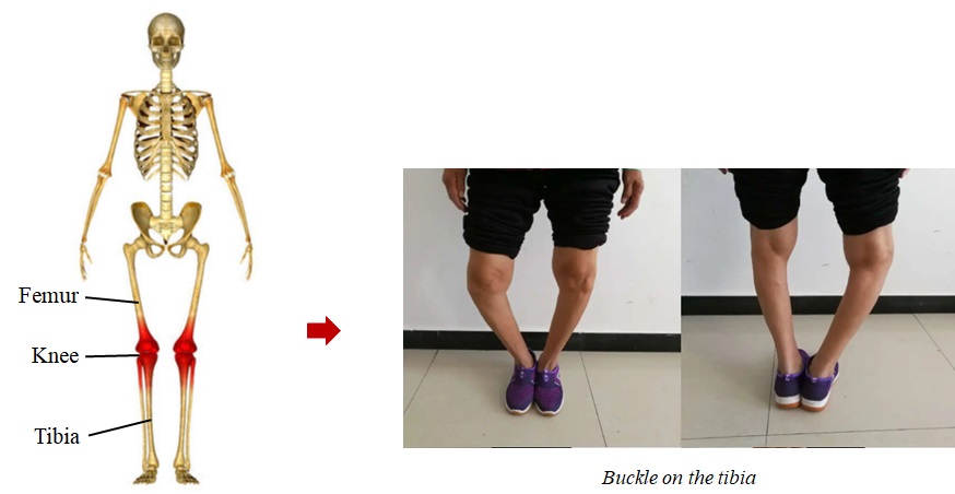
In addition, a common example of buckling in our body is the tibia which withstands the compression of our upper body and femur due to gravity and the support from the ground when we stand. In the normal situation, people’s tibias are straight and they don’t cause trouble to daily life. But in some special cases, for example, as shown in Fig. 3-5, the patient got a serious buckling on her tibia due to the pathological issues on her knees.
The contact stress in the knee is one of important subjects that researchers care about the most. There are two common methods to predict the stress.
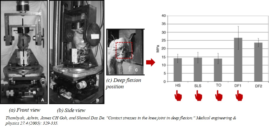
The first method is to conduct experiments using equipment and apparatus (Fig. 3-6). Thambyah and his colleagues tested the contact stresses in the knee joint in deep flexion using 5 cadavers. This figure shows the equipment that they used for the experiments. They applied loading conditions in various phases of walking and squatting to quasi-static mechanical testing on the cadaver knees. A thin-film electronic pressure transducer was inserted into the cadaver tibiofemoral joint space to measure force and area.
The means tested were those of peak contact stresses for the conditions simulating heel strike, single limb stance, toe-off positions and the deep flexion at 90 degrees and greater than 120 degrees positions. It was found that stresses peaked to 14MPa with a standard deviation of 2.5MPa. In deep flexion with 90 degrees, the peak stresses were significantly larger by over 80%, reaching the damage limits of cartilage.
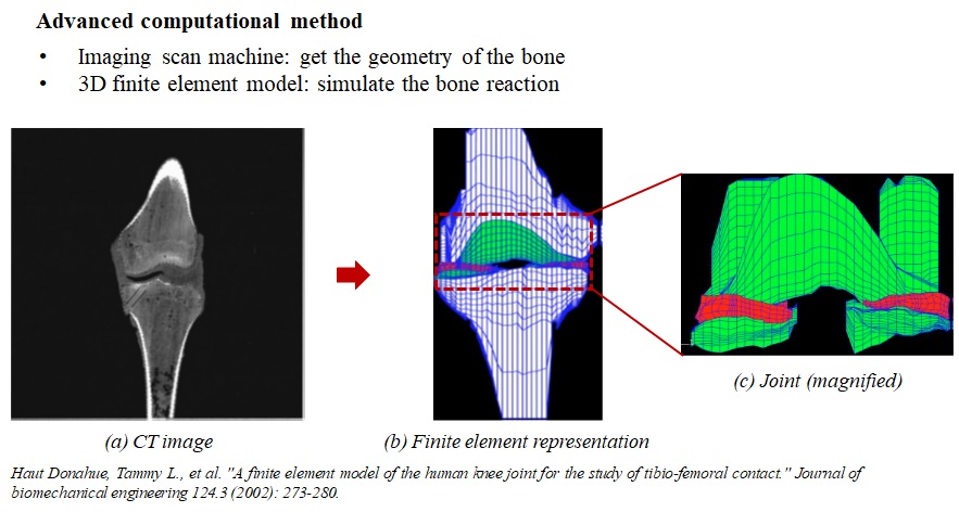
The second method is through computational models. Computational method is a popular way to analyze the bone response to any kind of loads. Usually, some imaging technologies, such as magnetic resonance imaging, also called MRI, reshaped digital calipers, and machine-controlled contact digitization, should be used to get the geometry of the bone. Then, the obtained bone geometry will be introduced to a computational software based on a mathematical approach called finite element method. In that case, researchers can simulate the bone reaction under loads which are of interest to them.
Donahue and her colleagues established a computational model of human knee joint to study the contact between tibia and femur (Fig. 3-7). They use a single right knee from a cadaveric specimen who was a male in the age of 30. After the preparation works, they use CT system to scan the knee in 0.5 mm increments in the frontal plane, from anterior to posterior at 0 degrees of flexion. The images of the slices were imported into Scion Image and the threshold was set to maximize contrast. At last, they get images in in a pixel size of 500 microns by 500 microns.
The three-dimensional solid model of the knee specimen was developed by importing the local coordinates from the digitized CT images and laser scanner into MSC/PATRAN. Input the coordinates into the computational software named ABAQUS, a simulation model of the entire tibio-femoral joint was constructed and meshed. Special attention is payed on the joint area. Care must be taken in establishing the computational model as it may cause convergence issue.
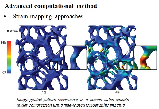
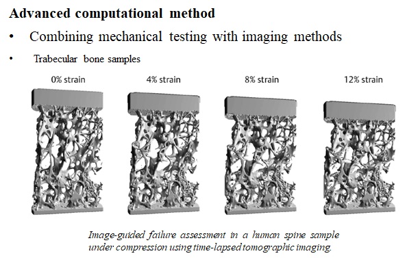
Whereas biomechanical testing provides detailed information on bone material properties, it fails in revealing local properties such as local deformations and strains. By combining mechanical testing with imaging methods, it has become possible to visualize and quantify bone deformations under load on various levels of structural organization. For trabecular bone samples, several deformations modes were found in human vertebral bone; some trabeculae bend, others buckle, and some are compressed as shown in Fig. 3-8.
Strain mapping is a mathematical technique to calculate how a bone or bone sample has deformed between two loading steps (Fig. 3-9).