
Stress: First and Second Piola-Kirchhoff Stress Tensors
Definitions
The Cauchy stress tensor defined previously, related area vectors  to traction vectors
  in the current state of deformation of a material object. The first and second Piola-Kirchhoff stress tensors extend the concept of “true” and “engineering” stress to the three-dimensional case and operate on area vectors in the undeformed state of the material. Assume that the area vector before any forces are applied to a continuum is equal to
  where
where  is the magnitude of the area and
  is the vector perpendicular to the underformed area. Assume that the forces applied lead to a deformation described by the linear mapping
  such that
  where
where  . Let the area vector after deformation be
  where
where  is the magnitude of the deformed area and
  is the vector perpendicular to the deformed area. Then, using Nanson’s formula:
![\[ (a)n=\det{(F)} (A)F^{-T}N \]](https://engcourses-uofa.ca/wp-content/ql-cache/quicklatex.com-329f636af9f49ba9673bb98cd5b0c197_l3.png "Rendered by QuickLaTeX.com")
The blue vectors in Figure 1 show a schematic of two undeformed unit area veoctors  and
and  (
( ) and their respective images
  and
and  after transformation by a linear mapping
  . After deformation, the force vector acting on an area with normal and magnitude
  is equal to
  . The first Piola-Kirchhoff stress tensor
  is defined as the tensor producing the same force vector
  when applied to the corresponding undeformed area vector :
![\[ f_N=f_n = (A)PN \]](https://engcourses-uofa.ca/wp-content/ql-cache/quicklatex.com-b4a811afe76855b4fdc4a567ddb61469_l3.png "Rendered by QuickLaTeX.com")
Using Nanson’s formula:
![\[ (A)PN=(a)\sigma^Tn=\det{(F)} (A)\sigma^TF^{-T}N \]](https://engcourses-uofa.ca/wp-content/ql-cache/quicklatex.com-01a60ac548c47b66b30b70d8852d01b6_l3.png "Rendered by QuickLaTeX.com")
Therefore,
![\[ PN=\det{(F)}\sigma^TF^{-T}N \]](https://engcourses-uofa.ca/wp-content/ql-cache/quicklatex.com-ee28e2c0c44354653d1ab8139531aff3_l3.png "Rendered by QuickLaTeX.com")
Which results in the following relationship between and  :
:
![\[ P=\det{(F)}\sigma^TF^{-T} \]](https://engcourses-uofa.ca/wp-content/ql-cache/quicklatex.com-d7c6c25e86272c67f3380a0d76453ccc_l3.png "Rendered by QuickLaTeX.com")
Note that the above relationship indicates that is not necessarily a symmetric matrix. The term “Nominal Stress Tensor” is sometimes used in the literature in reference to the first Piola-Kirchhoff stress or its transpose. The red vectors in Figure 1 show a schematic of the forces acting on the deformed area vectors and when viewed in the deformed configuration or when viewed in the undeformed configuration.
On the other hand, the second Piola-Kirchhoff stress tensor  is defined as the tensor producing a force vector
  when applied to the undeformed area vector .
  is sometimes termed the “pull-back” of the force vector . The relationship between and
  can be obtained as follows:
![\[ f2_N=(A)SN=F^{-1}f_n=(a)F^{-1}\sigma^Tn \]](https://engcourses-uofa.ca/wp-content/ql-cache/quicklatex.com-3a07f50c84480428d4d8419d3257dc66_l3.png "Rendered by QuickLaTeX.com")
Therefore:
![\[ (A)SN=(a)F^{-1}\sigma^Tn \]](https://engcourses-uofa.ca/wp-content/ql-cache/quicklatex.com-8ba8b12ef7ff18e760f4d7b4c8c4be49_l3.png "Rendered by QuickLaTeX.com")
Using Nanson’s formula:
![\[ (A)SN=(A)\det{(F)}F^{-1}\sigma^TF^{-T}N \]](https://engcourses-uofa.ca/wp-content/ql-cache/quicklatex.com-2a1780704d95c881a16b7d5231378ad9_l3.png "Rendered by QuickLaTeX.com")
Which results in the following relationship between and :
![\[ S=\det{(F)}F^{-1}\sigma^TF^{-T} \]](https://engcourses-uofa.ca/wp-content/ql-cache/quicklatex.com-bdd1fbf9eeba3d49b0be4fdae7a0e03b_l3.png "Rendered by QuickLaTeX.com")
Therefore is a symmetric tensor!
Notice that the relationship between and is:
![\[ S=F^{-1}P \]](https://engcourses-uofa.ca/wp-content/ql-cache/quicklatex.com-0f145a910783753ab2a5db2522cbc24c_l3.png "Rendered by QuickLaTeX.com")
The black vectors in Figure 1 show a schematic of the  and
and  which are the “pull-back” of the force vectors
  and
and  .
.
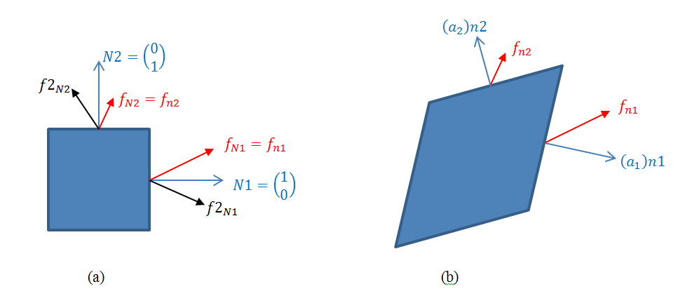
Figure 1. The force and area vectors on (a) the undeformed configuration, and (b) the deformed configuration.
The illustrative examples 1, 2, and 3 in the energy section can help clarify the difference between the three major stress tensors.
Example
Consider  . Assume that a region inside a material deforms according to the linear transformation described by:
![\[ F=\left(\begin{matrix}1.2 & 0.4\\0.4 & 1.2\end{matrix}\right) \]](https://engcourses-uofa.ca/wp-content/ql-cache/quicklatex.com-c1acd744d543d1296cafa23613e3bd40_l3.png "Rendered by QuickLaTeX.com")
Assume that the stress in the deformed configuration is described by the matrix:
![\[ \sigma=\left(\begin{matrix}5 & 2\\2 & 3\end{matrix}\right) \]](https://engcourses-uofa.ca/wp-content/ql-cache/quicklatex.com-ede93c1526b0c4314b5cb0f51037b804_l3.png "Rendered by QuickLaTeX.com")
Find:
- The area vectors after deformation of the two original unit areas with area vectors
 and
and  .
. - The first and second Piola-Kirchhoff stress matrices.
- The force vectors on the deformed planes whose undeformed unit area vectors are and using the Cauchy stress matrix.
- The force vectors produced by applying the first Piola-Kirchhoff stress tensor on the undeformed unit area vectors and .
- The force vectors produced by applying the second Piola-Kirchhoff stress tensor on the undeformed unit area vectors and .
Solution
Using Nanson’s formula (with ):
![\[\begin{split} (a_1)n1=\det{(F)} (A)F^{-T}N1=\left(\begin{array}{c} 1.2\\-0.4\end{array}\right)\\ (a_2)n2=\det{(F)} (A)F^{-T}N2=\left(\begin{array}{c} -0.4\\1.2\end{array}\right) \end{split} \]](https://engcourses-uofa.ca/wp-content/ql-cache/quicklatex.com-341a847c64729a3ec18328e8b730be59_l3.png "Rendered by QuickLaTeX.com")
Where  and
and  are the magnitudes of the “deformed” areas and
  and
and  are the corresponding normal vectors to the areas whose original normal vectors before deformation are and , respectively. The first and second Piola-Kirchhoff stress matrices and are:
![\[\begin{split} P=\det{(F)}\sigma^TF^{-T}=\left(\begin{matrix}5.2 & 0.4\\1.2 & 2.8\end{matrix}\right)\\ S=F^{-1}P=\left(\begin{matrix}4.5 & -0.5\\-0.5 & 2.5\end{matrix}\right) \end{split} \]](https://engcourses-uofa.ca/wp-content/ql-cache/quicklatex.com-fb68cc4da4efc541a9aaf02835c05401_l3.png "Rendered by QuickLaTeX.com")
The force vectors on the deformed area vectors and are:
![\[\begin{split} f_{n1}=(a_1)t_{n1}=(a_1)\sigma^T(n1)=\left(\begin{array}{c} 5.2\\1.2\end{array}\right)\\ f_{n2}=(a_2)t_{n2}=(a_2)\sigma^T(n2)=\left(\begin{array}{c} 0.4\\2.8\end{array}\right) \end{split} \]](https://engcourses-uofa.ca/wp-content/ql-cache/quicklatex.com-66e7f61e5544df2ee8196f6318d9060a_l3.png "Rendered by QuickLaTeX.com")
The force vectors on the original (undeformed) area vectors and obtained using the first Piola-Kirchoff stress are exactly the same ():
![\[\begin{split} f_{N1}=(A)P(N1)=\left(\begin{array}{c} 5.2\\1.2\end{array}\right)\\ f_{N2}=(A)P(N2)=\left(\begin{array}{c} 0.4\\2.8\end{array}\right) \end{split} \]](https://engcourses-uofa.ca/wp-content/ql-cache/quicklatex.com-d339a87aa9eb2c5cd24f6a436b3433cb_l3.png "Rendered by QuickLaTeX.com")
The force vectors on the original area vectors N1 and N2 when using the Second Piola-Kirchhoff stress ():
![\[\begin{split} f2_{N1}=(A)S(N1)=\left(\begin{array}{c} 4.5\\-0.5\end{array}\right)\\ f2_{N2}=(A)S(N2)=\left(\begin{array}{c} -0.5\\2.5\end{array}\right) \end{split} \]](https://engcourses-uofa.ca/wp-content/ql-cache/quicklatex.com-a64da081dcd9113317cf69619562fe2f_l3.png "Rendered by QuickLaTeX.com")
Notice that  and
and  . Figure 1 shows the deformation of an originally square object of unit length and the corresponding deformation of areas. The force vectors are also shown on the different areas before and after deformation. The Cauchy stress and the first Piola-Kirchhoff stress tensors produce the same
force vectors. The Cauchy stress matrix can intuitively be viewed as the force in the deformed configuration per unit area of the deformed configuration. The first Piola-Kirchhoff stress matrix can intuitively be viewed as the force in the deformed configuration per unit area of the undeformed configuration, while the second Piola-Kirchhoff stress can intuitively be viewed as the force in the undeformed configuration per unit area of the undeformed configuration. Notice that all these stress measures are equivalent, but they are useful for different applications.
F={{1.2,0.4},{0.4,1.2}};
Bx=Rectangle[{0,0}];
Bx2=GeometricTransformation[Bx,F];
Sigma={{5,2},{2,3}};
N1={1,0};
N2={0,1};
Farea=Det[F]*Transpose[Inverse[F]];
an1=Farea.N1;
an2=Farea.N2;
tn1=Transpose[Sigma].an1
tn2=Transpose[Sigma].an2
FirstPiola=Transpose[Sigma].Inverse[Transpose[F]]*Det[F];
SecondPiola=Inverse[F].FirstPiola;
TN1=FirstPiola.N1;
TN2=FirstPiola.N2;
STN1=SecondPiola.N1;
STN2=SecondPiola.N2;
Pt11=F.N1+1/2*F.N2;
Pt12=Pt11+an1;
Pt21=1/2*F.N1+F.N2;
Pt22=Pt21+an2;
ar1=Arrow[{Pt11,Pt12}];
ar2=Arrow[{Pt21,Pt22}];
A1dotted=Arrow[{Pt11,Pt11+{1,0}}];
A2dotted=Arrow[{Pt21,Pt21+{0,1}}];
A1=Arrow[{{1,0.5},{2,0.5}}];
A2=Arrow[{{0.5,1},{0.5,2}}];
artn1=Arrow[{Pt11,Pt11+1/10*tn1}];
artn2=Arrow[{Pt21,Pt21+1/10*tn2}];
arTN1=Arrow[{{1,0.5},{1,0.5}+1/10*TN1}];
arTN2=Arrow[{{0.5,1},{0.5,1}+1/10*TN2}];
arSTN1=Arrow[{{1,0.5},{1,0.5}+1/10*STN1}];
arSTN2=Arrow[{{0.5,1},{0.5,1}+1/10*STN2}];
Graphics[{Black,Bx,A1,A2,GrayLevel[0.1],arTN1,arTN2,GrayLevel[0.5],arSTN1,arSTN2}]
Graphics[{Black,Bx2,ar1,ar2,GrayLevel[0.1],artn1,artn2,Dashed,GrayLevel[0.5],A1dotted,A2dotted}]
In the following tool, change the values of and and watch how they affect the resulting deformation and forces acting on the different faces.