
Variational Principles: The Principle of Minimum Potential Energy for Conservative Systems in Equilibrium
A conservative system is defined as a system whose energy function is independent of the path between different deformation configurations, while a conservative force is defined as a force that exerts the same work to move a particle between two fixed points independent of the path taken. A conservative system would generally be composed of an elastic body acted upon by conservative forces. Forces arising due to gravity are in general conservative forces. On the other hand, nonconservative systems are those that usually contain frictional forces or nonelastic materials. For such systems, energy is lost during loading cycles that return the material back to its original position. For systems composed of elastic bodies and external forces that are conservative in nature, it will be shown that, provided a certain restriction on the constitutive equations for the elastic body, the state of static equilibrium corresponds to the state of minimum potential energy for the system.
Stable, Neutral, and Unstable Equilibria
For the purpose of illustration, the differences between stable, neutral, and unstable equilibrium states are often depicted though the use of schematics, such as Figure 1. In the three cases shown in the figure, the equations of equilibrium (sum of vertical forces is equal to zero) are achieved when the small cylinder is at position  . In Figure 1a, any perturbation (small change) in the position of the cylinder from point will not upset equilibrium because the cylinder will roll back to its equilibrium position. Clearly this is the position of “Stable Equilibrium”, and in fact, this is the position of the minimum potential energy of the system (Why?). In Figure 1b, the small cylinder is in equilibrium at any point on the flat surface since all those points correspond to the same potential energy; such equilibrium is termed “Neutral Equilibrium”. In Figure 1c, while the small cylinder is in static equilibrium on top of the larger cylinder, any small perturbation in the position of the smaller cylinder will upset equilibrium, and the small cylinder will roll away from the equilibrium position. It is clear that the equilibrium position in Figure 1c corresponds to the maximum potential energy of the system, and the system cannot sustain this position. Such type of equilibrium is termed “Unstable Equilibrium”.
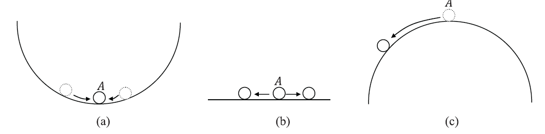
Figure 1. Types of equilibrium (a) Stable, (b) Neutral, and (c) Unstable equilibrium.
Potential Energy of a Conservative Mechanical System
The potential energy of a conservative mechanical system is defined as the internal elastic deformation (strain) energy stored inside the system minus the work done (or the potential energy lost) by the external forces acting on the system during a particular deformation. Expressions for the elastic strain energy in the special cases of linear elastic structures can be found here and will be used in the following.
The potential energy of a continuum when a displacement vector field  is applied is defined as follows:
(1) 
where  is the elastic deformation (elastic strain) energy function per unit volume of the deformed configuration,
  is the boundary traction vector, and
  is the body forces vector.
  is the work done (or potential energy lost) by the external forces when the continuum moves through the displacement vector .
If the continuum is made of a linear elastic isotropic material and if the deformations are small the potential energy of the system can be written as:
(2) 
Notice that for small deformations, the integration is done over the undeformed configuration and the small strain tensor is used as the energy conjugate for the Cauchy stress.
Similarly, the potential energy of an Euler Bernoulli (linear elastic isotropic) beam of length  is defined as follows:
(3) 
where  is the displacement of the Euler Bernoulli beam’s neutral axis,
  and
and  are the external point forces and moments,
  and
and  are the displacements and rotations corresponding to and respectively,
  and
and  are the numbers of external point forces and moments, and
  is the distributed lateral load on the beam.
For a small deformations beam under axial loading, the potential energy is defined as follows:
(4) 
where  is the distributed axial loading on the bar, and
  are the external forces and the corresponding displacements acting on the bar.
Principle of Stationary Potential Energy at Equilibrium
Equations 1, 2, 3, and 4 are defined for any arbitrary deformation. If the system is in equilibrium (i.e., the equilibrium equation is satisfied) and the deformation used to calculate the potential energy is the corresponding equilibrium deformation, then, we can use the principle of virtual work to show that the potential energy is stationary at the equilibrium deformation. We will show this for Equations 1 and 3, since the other two equations are just particular instances of the first equation. For Equation 1, assume that the mechanical system is in equilibrium under the action of the applied traction vector boundary field and body forces vector field , and the corresponding equilibrium displacement vector field is . We wish to show that a small variation in the displacement field  corresponds to a zero change in the potential energy. I.e.,
  . Let
. Let  be the strain field associated with , then, the potential energy associated with the displacement field
  is:
is:
![\[ PE(u+\Delta u)\approx PE(u)+\frac{\partial PE}{\partial u}\Delta u=PE(u)+\int_\Omega\! \sum_{i,j=1}^3\left(\frac{\partial \overline{U}}{\partial \varepsilon_{ij}}\Delta \varepsilon_{ij}\right)\,dx - \int_{\partial \Omega}\!t_n\cdot \Delta u\,dS - \int_\Omega\!\rho b\cdot \Delta u\,dx \]](https://engcourses-uofa.ca/wp-content/ql-cache/quicklatex.com-f5a3643a0881575bb4a98b9cdd51a29a_l3.png "Rendered by QuickLaTeX.com")
Using Equation 7 in the principle of virtual work we have:
![\[ \int_\Omega\! \sum_{i,j=1}^3\left(\frac{\partial \overline{U}}{\partial \varepsilon_{ij}}\Delta \varepsilon_{ij}\right)\,dx = \int_{\partial \Omega}\!t_n\cdot \Delta u\,dS + \int_\Omega\!\rho b\cdot \Delta u\,dx \]](https://engcourses-uofa.ca/wp-content/ql-cache/quicklatex.com-c01cda1df53dbbde7281e00386dc2825_l3.png "Rendered by QuickLaTeX.com")
Therefore,
![\[ PE(u+\Delta u)\approx PE(u) \]](https://engcourses-uofa.ca/wp-content/ql-cache/quicklatex.com-85c4024f9b024dd153e92318f555f5f7_l3.png "Rendered by QuickLaTeX.com")
i.e., the potential energy of a continuum that is in equilibrium is stationary. It is important to note that this result is a consequence of how the potential energy was defined. In fact, the potential energy was defined by integrating the equilibrium equation which results in its variation being zero at equilibrium.
Similarly, let be the equilibrium displacement of an Euler Bernoulli beam and let  be a variation of this equilibrium displacement associated and let
  be the associated rotation. Therefore,
![\[\begin{split} PE(y+\Delta y) & =\int_0^L\! \frac{EI}{2}\left(\frac{\mathrm{d}^2(y+\Delta y)}{\mathrm{d}X_1^2}\right)^2\,dX_1 - \int_0^L\!q(y+\Delta y)\,dX_1 - \sum_{i=1}^nF_i(y_i+\Delta y_i)-\sum_{j=1}^mM_j(\theta_j+\Delta\theta_j)\\ & \approx PE(y) + \int_0^L\! \frac{EI}{2}\frac{\mathrm{d}^2(y)}{\mathrm{d}X_1^2}\frac{\mathrm{d}^2(\Delta y)}{\mathrm{d}X_1^2}\,dX_1 - \int_0^L\!q(\Delta y)\,dX_1 - \sum_{i=1}^nF_i(\Delta y_i)-\sum_{j=1}^mM_j(\Delta\theta_j) \end{split} \]](https://engcourses-uofa.ca/wp-content/ql-cache/quicklatex.com-cccf1b691eb00a6cd1daa13a7144c4df_l3.png "Rendered by QuickLaTeX.com")
Using Equation 8 in the principle of virtual work we have:
![\[ \int_0^L\! \frac{EI}{2}\frac{\mathrm{d}^2(y)}{\mathrm{d}X_1^2}\frac{\mathrm{d}^2(\Delta y)}{\mathrm{d}X_1^2}\,dX_1 = \int_0^L\!q(\Delta y)\,dX_1 + \sum_{i=1}^nF_i(\Delta y_i)+\sum_{j=1}^mM_j(\Delta\theta_j) \]](https://engcourses-uofa.ca/wp-content/ql-cache/quicklatex.com-5aa7e11c56f5e0bd191c4237cdca234d_l3.png "Rendered by QuickLaTeX.com")
Therefore,
![\[ PE(y+\Delta y)\approx PE(y) \]](https://engcourses-uofa.ca/wp-content/ql-cache/quicklatex.com-c9402ad3aa41b71a53bd8f211d0b3980_l3.png "Rendered by QuickLaTeX.com")
i.e,. the potential energy of an Euler Bernoulli beam that is in equilibrium is stationary.
Principle of Minimum Potential Energy at Equilibrium
Since the potential energy of a conservative mechanical system at equilibrium is stationary, the value corresponding to the equilibrium displacement is either minimum, maximum, or an inflection point. Stable equilibrium is defined as the equilibrium corresponding to minimum potential energy (See Figure 1). If the external forces are not functions of the applied displacement then the second variation of the potential energy of a continuum is given by:
![\[ \frac{\partial^2 PE}{\partial \varepsilon_{ij}\partial \varepsilon_{kl}}=\int_\Omega \! \frac{\partial^2 \overline{U}}{\partial \varepsilon_{ij}\partial \varepsilon_{kl}}\,dx \]](https://engcourses-uofa.ca/wp-content/ql-cache/quicklatex.com-9bb299e6c0c6b199cff2b6266981bcec_l3.png "Rendered by QuickLaTeX.com")
For the system to be in stable equilibrium, the left hand side has to be greater than zero at equilibrium. This imposes a severe mathematical restriction on the strain energy function such that a stable equilibrium is always achieved; this mathematical restriction is called positive definiteness. Fortunately, for small deformations linear elastic materials, such condition is readily satisfied when the material constants follow the restrictions imposed on the elastic moduli. Recall that for the linear isotropic material law to be positive definite, Young’s modulus  and Poisson’s ratio have the following restrictions:
  and
and  .
.
Similarly, if the external forces are not functions of the applied displacement, and setting  then the second variation of the potential energy of an Euler Bernoulli beam is given by:
![\[ \frac{\partial^2 PE}{\partial g^2}=\int_0^L \! EI\,dX_1 \]](https://engcourses-uofa.ca/wp-content/ql-cache/quicklatex.com-b5c0e686681f909937f28e1b8005e270_l3.png "Rendered by QuickLaTeX.com")
Since  , therefore, the equilibrium of an Euler Bernoulli beam under lateral loads with a positive Young’s modulus is always a stable equilibrium.
Linear Elastic Materials with Small Deformations
For linear elastic small deformations materials when the infinitesimal strain matrix is used as the strain measure, the positive definiteness of the internal energy is satisfied. The strain energy function is quadratic, and thus, it is indeed convex in the variables  . For such materials, rigid body displacements (but not necessarily rotations!)
result in zero strain components and thus are not accompanied by a change in the internal energy. For linear elastic small deformations, the potential energy is indeed minimum at equilibrium when the infinitesimal strain matrix is used. It should also be noted that in the derivation in the previous section, the components in the continuum potential energy were taken as gradients with respect to the deformed configuration coordinate system. However, the infinitesimal strain tensor is in fact defined as gradients with respect to the undeformed configuration coordinate system. For small deformations, the following approximation is traditionally used:
![\[ \varepsilon_{ij}=\frac{1}{2}\left(\frac{\partial u_i}{\partial X_j}+\frac{\partial u_j}{\partial X_i}\right)\approx\frac{1}{2}\left(\frac{\partial u_i}{\partial x_j}+\frac{\partial u_j}{\partial x_i}\right) \]](https://engcourses-uofa.ca/wp-content/ql-cache/quicklatex.com-b51c1182edd1bb5cfd8895e62e6f5ce0_l3.png "Rendered by QuickLaTeX.com")
Such approximation is valid only if the deformation gradient is small enough such that it can be approximated by the identity matrix  plus a matrix of small numbers
  :
:
![\[ \frac{\partial u}{\partial X}=\frac{\partial u}{\partial x}\frac{\partial x}{\partial X}=\frac{\partial u}{\partial x}(I+\delta)\approx \frac{\partial u}{\partial x} \]](https://engcourses-uofa.ca/wp-content/ql-cache/quicklatex.com-f8e05f40be7d1832ff1e96b80d643886_l3.png "Rendered by QuickLaTeX.com")
The principle of minimum potential energy for linear elastic small deformation materials is very successful in finding solutions for problems in solid mechanics engineering applications. However, the principle of minimum potential energy when the infinitesimal strain tensor is used can fail in predicting phenomena like buckling, since buckling involves large rotations. In this case, the use of the infinitesimal strain matrix is erroneous since it predicts nonzero values for the strain components when large rotations are encountered. These erroneous nonzero strain values can inhibit predicting certain types of mechanical behaviour accompanied by large rotations.
Large Deformations
In large deformations, the expressions for the virtual work and the second derivative of the potential energy of the system are derived by defining  using the deformed coordinates:
![\[ \varepsilon_{ij}^*=\frac{1}{2}\left(\frac{\partial u_i^*}{\partial x_j}+\frac{\partial u_j^*}{\partial x_i}\right) \]](https://engcourses-uofa.ca/wp-content/ql-cache/quicklatex.com-61996360db5e19760803c8af78c8724e_l3.png "Rendered by QuickLaTeX.com")
Phenomena like buckling, which are accompanied by large rotations without any change in the internal energy, can be modelled using the principle of virtual work since, during rotations, the terms are all equal to zero since  (For pure rotation, the stretch rate
  of the velocity gradient is equal to zero). Constitutive models for large deformation hyperelastic materials are either given in terms of the principal stretches
  ,
,  , and
, and  . Such materials have a strain energy potential that is a function in the principal stretches , , and , and thus, large rotations are accompanied by zero strain energy. If the post-buckling behaviour is stable, then it can be predicted using the principle of minimum potential energy at equilibrium for a continuum with large deformations.
Example
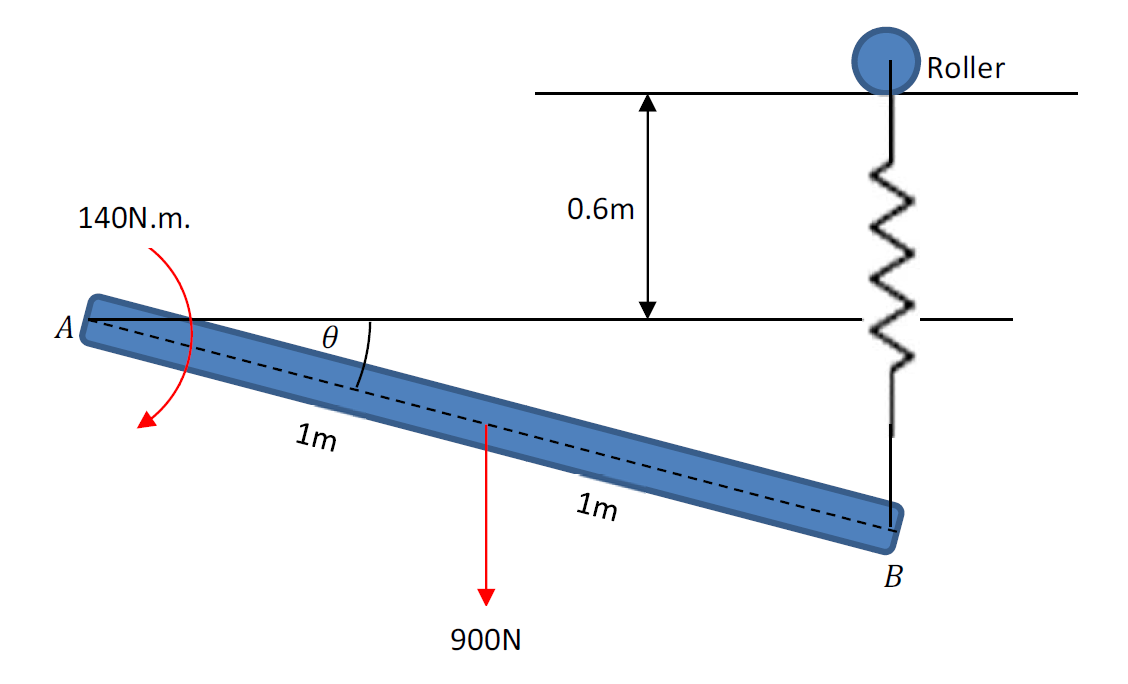
The shown rod supports a weight of 900N and is pinned at point . It is also subjected to a moment of value 140N.m. Determine the possible equilibrium positions described by the angle  and determine whether they are stable or not. The spring has an unstretched length of 0.6m and a stiffness
  .
.
Solution
The equilibrium equation (sum of moments around point ) is given by:
![\[ M_{@A}=-140-900\cos{\theta}+750 (2\sin{\theta})(2\cos{\theta})=-140-900\cos{\theta}+3000 \sin{\theta}\cos{\theta}=0 \]](https://engcourses-uofa.ca/wp-content/ql-cache/quicklatex.com-5b1bda9781d7c6f8b2e5bfe8ef324ab4_l3.png "Rendered by QuickLaTeX.com")
Solving the above equation leads to four possible angles at which the rod is in equilibrium:
![\[ \theta_1=19.6^\circ \qquad \theta_2=87.27^\circ\qquad \theta_3=164.61^\circ \qquad \theta_4=268.53^\circ \]](https://engcourses-uofa.ca/wp-content/ql-cache/quicklatex.com-2e13c9b971ebfe41720114b6585b7bd8_l3.png "Rendered by QuickLaTeX.com")
The same solution can be found if we write the potential energy of the system and find the angle that would minimize the expression for the potential energy:
![\[ PE=\frac{1}{2}750 (2\sin{\theta})^2-900\sin{\theta}-140\theta \]](https://engcourses-uofa.ca/wp-content/ql-cache/quicklatex.com-c37183ee4505ea36934637cc35b5b4c7_l3.png "Rendered by QuickLaTeX.com")
To find the equilibrium angle, the rate of change of the potential energy with respect to is equated to zero:
![\[ \frac{\partial PE}{\partial \theta}=-140-900\cos{\theta}+3,000 \sin{\theta}\cos{\theta}=0 \]](https://engcourses-uofa.ca/wp-content/ql-cache/quicklatex.com-3e6c7791bb873890a4c5f284047502f8_l3.png "Rendered by QuickLaTeX.com")
which is exactly the equilibrium equation. To find out whether the equilibrium is stable or not at each of the possible four angles of equilibrium the second derivative is evaluated:
![\[ \frac{\partial^2 PE}{\partial \theta^2}=3000 (\cos{\theta})^2+900 \sin{\theta} - 3000 (\sin{\theta})^2 \]](https://engcourses-uofa.ca/wp-content/ql-cache/quicklatex.com-c93ac89bca017a25366c3d280cb7a07b_l3.png "Rendered by QuickLaTeX.com")
By substituting the possible angles of equilibrium in the above equation we get:
![\[ \frac{\partial^2 PE}{\partial \theta^2}\bigg|_{\theta=\theta_1}=845.6 \qquad \frac{\partial^2 PE}{\partial \theta^2}\bigg|_{\theta=\theta_2}=-59.6 \qquad \frac{\partial^2 PE}{\partial \theta^2}\bigg|_{\theta=\theta_3}=-1532.3 \qquad \frac{\partial^2 PE}{\partial \theta^2}\bigg|_{\theta=\theta_4}=-3863 \]](https://engcourses-uofa.ca/wp-content/ql-cache/quicklatex.com-77cd35c6a1f5cbc1132fcd88bea7ed2c_l3.png "Rendered by QuickLaTeX.com")
Therefore, only  is a stable equilibrium position.
Equil = -140.0 – 900 Cos[th] + 750*4*Cos[th]*Sin[th];
s = Solve[Equil == 0, {th}] th1 = (th /. s[[2]])/Degree
th2 = (th /. s[[3]])/Degree
th3 = (th /. s[[4]])/Degree
th4 = (th /. s[[1]])/Degree
th4 = 360 + (th /. s[[1]])/Degree
(*PE*)
PE = 750/2*(2 Sin[th])^2 – 140*th – 900 Sin[th];
Eq1 = D[PE, th] D2PE = D[PE, {th, 2}] D2PE /. {th -> th1}
D2PE /. {th -> th2}
D2PE /. {th -> th3}
D2PE /. {th -> th4}