Engineering at Alberta Courses » The Deformation Gradient

Displacement and Strain: The Deformation Gradient

Definitions:

For a general 3D deformation of an object, local strains can be measured by comparing the “length” between two neighbouring points before and after deformation. Thus, we are interested in tracking lines or curves on the reference and deformed configuration. The restrictions on the possible position functions $f$ (especially being differentiable) allow such comparisons and calculation as follows:
We first assume a material curve inside the reference and deformed configurations by assuming a parameter $\xi\in\mathbb{R}$ that defines the curve (Figure 1). The position in the reference and deformed configurations respectively are given by $X(\xi)$ and $x(\xi,t)$ where $t$ refers to time:

$X= \left(\begin{array}{c} X_1(\xi)\\ X_2(\xi)\\X_3(\xi) \end{array}\right)\qquad x= \left(\begin{array}{c} x_1(\xi,t)\\ x_2(\xi,t)\\x_3(\xi,t) \end{array}\right)$

The tangents to the material curves at a point given by a particular value for the parameter $\xi$ in the reference and deformed configurations are denoted $N\in\mathbb{R}^3$ and $n\in\mathbb{R}^3$ respectively (Figure 1) and given by:

$N=\frac{\partial X}{\partial \xi}= \left(\begin{array}{c} \frac{\partial X_1}{\partial \xi}\\ \frac{\partial X_2}{\partial \xi}\\\frac{\partial X_3}{\partial \xi} \end{array}\right)\qquad n=\frac{\partial x}{\partial \xi}=\frac{\partial x}{\partial X}\frac{\partial X}{\partial \xi}= \left(\begin{array}{ccc} \frac{\partial x_1}{\partial X_1} & \frac{\partial x_1}{\partial X_2} & \frac{\partial x_1}{\partial X_3}\\ \frac{\partial x_2}{\partial X_1} & \frac{\partial x_2}{\partial X_2} & \frac{\partial x_2}{\partial X_3}\\ \frac{\partial x_3}{\partial X_1} & \frac{\partial x_3}{\partial X_2} & \frac{\partial x_3}{\partial X_3} \end{array}\right) \left(\begin{array}{c} \frac{\partial X_1}{\partial \xi}\\ \frac{\partial X_2}{\partial \xi}\\\frac{\partial X_3}{\partial \xi} \end{array}\right)$

The matrix $F$ :

$F=\left(\begin{array}{ccc} \frac{\partial x_1}{\partial X_1} & \frac{\partial x_1}{\partial X_2} & \frac{\partial x_1}{\partial X_3}\\ \frac{\partial x_2}{\partial X_1} & \frac{\partial x_2}{\partial X_2} & \frac{\partial x_2}{\partial X_3}\\ \frac{\partial x_3}{\partial X_1} & \frac{\partial x_3}{\partial X_2} & \frac{\partial x_3}{\partial X_3} \end{array}\right)$

is denoted the “Deformation Gradient” and contains all the required local information about the changes in length, volumes and angles due to the deformation as follows:

A tangent vector $N$ in the reference configuration is deformed into the tangent vector $n$ . The two vectors are related using the deformation gradient tensor $F$ :
$n = FN$
The ratio between the local volume of the deformed configuration to the local volume in the reference configuration is equal to the determinant of $F$ .
If an infinitesimal area vector is termed $(da) n$ and $(dA) N$ in the deformed and reference configurations respectively, with $da$ and $dA$ in $\mathbb{R}$ being the magnitudes of the area while $n$ and $N$ are the unit vectors perpendicular to the corresponding areas, then using Nanson’s formula shown in the section on the determinant of matrices $\mathbb{M}^3$ , the relationship between them is given by:
$(da) n = \det(F)(dA)F^{-T}N$
An isochoric deformation is a deformation preserving local volume, i.e., $\det(F)=1$ at every point.
A deformation is called homogeneous if $F$ is constant at every point, i.e., $F$ is not a function of position. Otherwise, the deformation is called non-homogeneous.
The physical restrictions of possible deformations force the $\det(F)$ to be always positive. (why?)

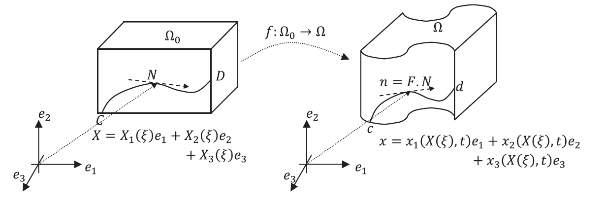
Tangents to material curves in the reference and deformed configurations. Points C and D in the reference configuration correspond to points c and d in the deformed configuration.

Figure 1. Tangents to material curves in the reference and deformed configurations. Points $C$ and $D$ in the reference configuration correspond to points $c$ and $d$ in the deformed configuration.

The Polar Decomposition of the Deformation Gradient:

One of the general results of linear algebra is the Polar Decomposition of matrices which states the following. Any matrix of real numbers $F\in\mathbb{M}^n$ can be decomposed into two matrices multiplied by each other $F=QU$ such that $Q\in\mathbb{M}^n$ is an orthogonal matrix and $U\in\mathbb{M}^n$ is a semi-positive definite symmetric matrix. In particular, if $\det(F)>0$ , then we can find a rotation matrices $R\in\mathbb{M}^n$ and two positive-definite symmetric matrices $U\in\mathbb{M}^n$ and $V\in\mathbb{M}^n$ such that

$F=RU=VR$

For continuum mechanics applications, $U$ and $V$ are termed the right and left stretch tensors respectively. The first equality is termed the “right” polar decomposition while the second is called the “left”. The proof of the above statement presented here is based on the two books:

Ciarlet, P.G. (2004). Mathematical Elasticity. Volume 1: Three Dimensional Elasticity. Elsevier Ltd.
Chadwick, P. (1999). Continuum Mechanics. Concise Theory and Problems. Dover Publications Inc.

and it will be presented using several statements.

Statement 1:

Let $F\in\mathbb{M}^3$ be such that $\det(F)>0$ . Then, the matrices $C=F^TF$ and $B=FF^T$ are positive definite symmetric matrices.

Proof:

The symmetry of $C$ and $B$ is straightforward as follows:

$C^T=(F^TF)^T=F^T{F^T}^T=F^TF=C\qquad B^T=(FF^T)^T={F^T}^TF^T=FF^T=B$

Also, since $\det(F)>0$ , therefore: $\forall x\in\mathbb{R}^n/\{0\}$ (i.e., $x\neq 0$ ) we have $Fx\neq 0$ . Therefore, $\|Fx\|^2=Fx\cdot Fx=x\cdot F^TFx=x\cdot Cx>0$ . Therefore, $C$ is positive definite.
Similarly, it can be shown that $B$ is positive definite.

$\blacksquare$

Statement 2:

Let $M\in\mathbb{M}^3$ be such that $M$ is a positive definite symmetric matrix. Show that there exists a unique square root positive-definite symmetric matrix for $M$ (denoted by $M^{1/2}$ such that $M=M^{1/2}M^{1/2}$ .

Proof:

The existence of a square root is straightforward. As per the results in the symmetric tensors section, we can choose a coordinate system such that $M$ is diagonal with three positive real numbers $M_1, M_2$ and $M_3$ in the diagonal:

$M=\left(\begin{array}{ccc} M_1 & 0 & 0\\ 0 & M_2 & 0\\ 0 & 0 & M_3 \end{array} \right)$

By setting $\lambda_1=\sqrt{M_1}, \lambda_2=\sqrt{M_2}$ and $\lambda_3=\sqrt{M_3}$ then:

$M^{1/2}=\left(\begin{array}{ccc} \lambda_1 & 0 & 0\\ 0 & \lambda_2 & 0\\ 0 & 0 & \lambda_3 \end{array} \right)$

and it is straightforward to show that: $M=M^{1/2}M^{1/2}$ in any coordinate system.

The uniqueness of $M^{1/2}$ can be shown using contradiction by assuming that there are two different positive definite square roots $U_1$ and $U_2$ such that

$M=U_1U_1=U_2U_2$

$M$ is a positive-definite symmetric matrix with positive eigenvalue $M_1, M_2$ and $M_3$ . Let $p\in\mathbb{R}^3$ be the eigenvector associated with $M_1$ , therefore:

$Mp=M_1p\Rightarrow U_1U_1p=M_1p=\lambda_1^2p\Rightarrow (U_1+\lambda_1I)(U_1-\lambda_1I)p=0$

Since by assumption, $U_1$ is positive definite, therefore $\lambda_1$ is an eigenvalue of $U_1$ associated with the eigenvector $p$ ; otherwise, $-\lambda_1$ is an eigenvalue of $U_1$ which contradicts that it is positive definite. This applies to $U_2$ as well and therefore, $U_1$ and $U_2$ are positive definite symmetric matrices that share the same eigenvalues and eigenvectors, therefore, they are identical (why?).

$\blacksquare$

Notice that a positive definite symmetric matrix can have various “square roots”, however, there is only one unique square root that is also a positive definite symmetric matrix. For example, consider the matrix:

$M=\left(\begin{array}{ccc} 4 & 0 & 0\\ 0 & 4 & 0\\ 0 & 0 & 1 \end{array} \right)$

The unique positive definite symmetric square root of $M$ is:

$M^{1/2}=\left(\begin{array}{ccc} 2 & 0 & 0\\ 0 & 2 & 0\\ 0 & 0 & 1 \end{array} \right)$

However, the following symmetric matrix $A$ is also a square root of $M$ , nevertheless, it is NOT positive-definite:

$A=\sqrt{2}\left(\begin{array}{ccc} 1 & 1 & 0\\ 1 & -1 & 0\\ 0 & 0 & 1/\sqrt{2} \end{array} \right)$

Verify that $M=AA$ and $A$ is NOT positive-definite.

Statement 3:

Let $F\in\mathbb{M}^3$ be such that $\det(F)>0$ . Show that there exists $F$ can be uniquely decomposed into:

$F=RU=VR$

where, $U=(F^TF)^{1/2}$ and $V=(FF^T)^{1/2}$ are positive-definite symmetric matrices while $R\in\mathbb{M}^3$ is a rotation matrix.

Proof:

From the statements 1 and 2 above, $U$ and $V$ are unique positive definite symmetric matrices, therefore, they are invertible (why?). Let

$R=FU^{-1}\qquad S=V^{-1}F$

Both $R$ and $S$ are invertible, (why?). In addition:

$RR^T=FU^{-1}U^{-1}F^T=F(F^TF)^{-1}F^T=FF^{-1}(F)^{-T}F^T=I$

and

$S^TS=F^TV^{-1}V^{-1}F=F^T(FF^T)^{-1}F^T=F^TF^{-T}F^{-1}F=I$

We also have: $\det(U)^2=\det(F)\det(F^T)$ and $\det(U)>0$ , therefore, $\det(U)=\det(F)$ . Therefore, $\det(R)=1$ . Similarly, $\det(S)=1$ . Therefore, both, $R$ and $S$ are rotation matrices.
Since $U$ and $V$ are invertible and unique, $R$ and $S$ are also unique. We can show this by contradiction, by assuming that:

$F=RU=R'U$

Therefore:

$RUU^{-1}=R'UU^{-1}\Rightarrow R=R'$

The same argument applies for $S$ .

Finally, it is required to show that $S=R$ , indeed:

$F=RU=VS=IVS=(S^TS)VS=S(S^TVS)$

However, $S^TVS$ is a positive definite symmetric matrix (why?), and since the decomposition $F=RU$ is unique, therefore,

$S=R\qquad U=R^TVR$

$\blacksquare$

Statement 4:

$V$ and $U$ share the same eigenvalues and their eigenvectors differ by the rotation $R$

Proof:

Assuming that $\lambda_1$ is an eigenvalue of $V$ with the corresponding eigenvector $n_1$ , then:

$Vn_1=\lambda_1 n_1 \Rightarrow \left(RUR^T\right)n_1=\lambda_1 n_1 \Rightarrow \left(R^TRU\right)\left(R^Tn_1\right)=\lambda_1\left(R^Tn_1\right)\Rightarrow U\left(R^Tn_1\right)=\lambda_1\left(R^Tn_1\right)$

Therefore, $\lambda_1$ is an eigenvalue of $U$ while $R^T n_1$ is the associated eigenvector.

Similarly, if $\lambda_2$ is an eigenvalue of $U$ with the corresponding eigenvector $N_2$ , then:

$UN_2=\lambda_2 n_2 \Rightarrow \left(R^TVR\right)N_2=\lambda_2 N_2 \Rightarrow \left(RR^TV\right)\left(RN_2\right)=\lambda_2\left(RN_2\right)\Rightarrow U\left(RN_2\right)=\lambda_2\left(RN_2\right)$

Therefore, $\lambda_2$ is an eigenvalue of $V$ while $R N_2$ is the associated eigenvector.
Assuming that $\lambda_1$ , $\lambda_2$ and $\lambda_3$ are the eigenvalues of $U$ and $V$ , $N_1$ , $N_2$ , and $N_3$ are the associated eigenvectors of $U$ , while $n_1$ , $n_2$ , and $n_3$ are the associated eigenvectors of $V$ , then $U$ and $V$ admit the representations (see the section about the representation of symmetric matrices):

$U=\lambda_1 (N_1\otimes N_1)+\lambda_2 (N_2\otimes N_2)+\lambda_3 (N_3\otimes N_3)$

$V=\lambda_1 (n_1\otimes n_1)+\lambda_2 (n_2\otimes n_2)+\lambda_3 (n_3\otimes n_3)$

and $\forall i\in\{1,2,3\}$ :

$n_i=RN_i$

$\blacksquare$

Physical Interpretation:

The unique decomposition of the deformation gradient F into a rotation and a stretch indicates that any smooth deformation can be decomposed at any point inside the continuum body into a unique stretch described by $U$ followed by a unique rotation described by $R$ . For example, a circle representing the directions of all the vectors in $\mathbb{R}^2$ is deformed into an ellipse under the action of $F:\mathbb{R}^2\rightarrow\mathbb{R}^2$ where $\det(F)>0$ . The decomposition $F=RU$ is schematically shown by first stretching the circle into an ellipse whose major axes are the eigenvectors of $U$ followed by a rotation of the ellipse through the matrix $R$ . The decomposition $F=VR$ represents rotating the circle through the matrix $R$ and then stretching the circle into an ellipse whose major axes are the eigenvectors of $V$ . Notice that the eigenvectors of V and the eigenvectors of U differ by a mere rotation. In the following tool, change the values of the four components of the matrix $F\in\mathbb{R}^2$ . The code first ensures that $\det(F)>0$ . Once this condition is satisfied, the tool draws the two steps of the right polar decomposition in the first row and then the steps of the left polar decomposition in the second row. In the first image on the first row, the arrows indicate the eigenvectors of $U$ . The arrows are shown to deform but keep their direction in the second image of the first row. Then, after applying the rotation, the arrows rotate in the third image of the first row. In the second image of the second row, the arrows are rotated with the matrix $R$ without any change in length. Then, they are deformed using the matrix $V$ in the third image of the second row.

The Singular-Value Decomposition of the Deformation Gradient:

One of the general results of linear algebra is the Singular-Value Decomposition of real or complex matrices. When the statement is applied to a matrix $F\in\mathbb{M}^3$ with $\det(F)>0$ it states that $F$ can be decomposed as follows:

$F=PDQ^T$

Where, $P$ and $Q$ are rotation matrices while the matrix $D$ is a diagonal matrix with positive diagonal entries. The singular-value decomposition follows immediately from the previous section on the polar decomposition of the deformation gradient. By setting $F=RU$ and realizing that $U$ is a positive definite symmetric matrix, then using the spectral form of symmetric tensors $U$ can be decomposed such that $U=QDQ^T$ where $D$ is a diagonal matrix whose diagonal entries are positive and $Q$ is a rotation matrix whose columns are the normalized eigenvectors of $U$ (The rows of $Q^T$ are the normalized eigenvectors of $U$ ). In particular, they are the square roots of the eigenvalues of the positive definite symmetric matrix $F^TF$ .
Therefore:

$F=RU=RQDQ^T$

By setting $P=RQ$ we get the required result:

$F=PDQ^T$

The following tool calculates the polar decomposition and the singular value decomposition of a matrix $F\in\mathbb{R}^3$ . Enter the values for the components of $F$ and the tool calculates all the required matrices after checking that $\det(F)>0$ .

The Right Cauchy-Green Deformation Tensor:

The tensor $C=F^TF$ is termed the right Cauchy-Green deformation tensor. As shown above, it is a positive definite symmetric matrix, thus, it has three positive real eigenvalues and three perpendicular eigenvectors. It also has a unique positive square root $U^2=C$ (See statement 2 above) such that $U$ has the same eigenvectors, while the eigenvalues of $U$ are the positive square roots of the eigenvalues of $C$ . Denote $\lambda_1^2$ , $\lambda_2^2$ , and $\lambda_3^2$ as the eigenvalues of $C$ with the corresponding eigenvectors $N_1$ , $N_2$ and $N_3$ , then $C$ , $U$ and $F$ admit the representations (see the section about the representation of symmetric matrices):

$C=\lambda_1^2 (N_1\otimes N_1)+\lambda_2^2 (N_2\otimes N_2)+\lambda_3^2 (N_3\otimes N_3)$

$U=\lambda_1 (N_1\otimes N_1)+\lambda_2 (N_2\otimes N_2)+\lambda_3 (N_3\otimes N_3)$

$F=RU=R\left(\lambda_1 (N_1\otimes N_1)+\lambda_2 (N_2\otimes N_2)+\lambda_3 (N_3\otimes N_3)\right)$

It is worth noting that the last expression for $F$ is equivalent to the singular-value decomposition of $F$ described above. The singular-value decomposition, $F=RQDQ^T$ where $Q$ is a rotation matrix whose columns are the eigenvectors of $U$ , is more convenient for component calculations, while the last expression with tensor product is much more useful for formula manipulation.

The Left Cauchy-Green Deformation Tensor:

The tensor $B=FF^T$ is termed the left Cauchy-Green deformation tensor. As shown above, it is a positive definite symmetric matrix, thus, it has three positive real eigenvalues and three perpendicular eigenvectors. It also has a unique positive square root $V^2=C$ (See statement 2 above) such that $V$ has the same eigenvectors, while the eigenvalues of $V$ are the positive square roots of the eigenvalues of $B$ . From statement 2 and statement 4 above, the eigenvalues of $B=V^2$ and $C=U^2$ are the same while the eigenvectors differ by the rotation $R$ (why?). Denote $\lambda_1^2$ , $\lambda_2^2$ , and $\lambda_3^2$ as the eigenvalues of $B$ with the corresponding eigenvectors $n_1$ , $n_2$ and $n_3$ , then $B$ , $V$ and $F$ admit the representations (see the section about the representation of symmetric matrices):