Approximate Methods: Rayleigh Ritz Method
The Rayleigh Ritz method is a classical approximate method to find the displacement function of an object such that the it is in equilibrium with the externally applied loads. It is regarded as an ancestor of the widely used Finite Element Method (FEM). The Rayleigh Ritz method relies on the principle of minimum potential energy for conservative systems. The method involves assuming a form or a shape for the unknown displacement functions, and thus, the displacement functions would have a few unknown parameters. These assumed shape functions are termed Trial Functions. Afterwards, the potential energy function of the system is written in terms of those few parameters, and the values of those parameters that would minimize the potential energy function of the system are calculated. Mathematically speaking, we assume that the unknown displacement function  is a member of a certain space of functions; for example, we can assume that
  where
where  is the set of all the possible vector valued linear functions defined on the body represented by the set
  . With this assumption, we restrict the possible solutions to those in the form
  , and thus, the unknown parameters are restricted to the matrix
  , which in this particular example, has nine components. Finally, the nine components that would minimize the potential-energy function are obtained. The method will be illustrated using various one-dimensional examples.
Bars under Axial Loads
The Rayleigh Ritz method seeks to find an approximate solution to minimize the potential energy of the system. For plane bars under axial loading, the unknown displacement function is  . In this case, the potential energy of the system has the following form (See beams under axial loads and energy expressions):
![\[ PE=\mbox{Total Strain Energy} - W=\int\!\frac{EA}{2}\left(\frac{\mathrm{d}u_1}{\mathrm{d}X_1}\right)^2 \,\mathrm{d}X_1 - W \]](https://engcourses-uofa.ca/wp-content/ql-cache/quicklatex.com-81b0bf361272bfdce2707eb9a7bc1dc8_l3.png "Rendered by QuickLaTeX.com")
where  is Young’s modulus,
  is the cross sectional area, and
  is the work done by all the external forces acting on the bar (concentrated forces and distributed loads). To obtain an approximate solution for , a trial function of a finite number of unknowns is first selected. Then, this trial function has to satisfy the “essential” boundary conditions, which are those boundary conditions that would satisfy the physical stability of the system. In the case of bars under axial loads, the trial function has to satisfy the displacement boundary conditions. The following examples show the method for different external loads, and bar configurations.
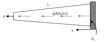
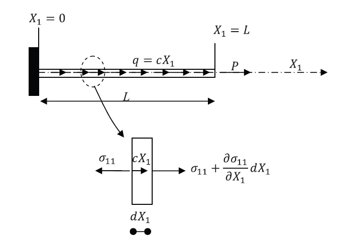
Example 1: A Bar under Axial Forces
Let a bar with a length  and a constant cross sectional area be aligned with the coordinate axis
  . Assume that the bar is subjected to a horizontal body force (in the direction of the axis )
  units of force/unit length where
  is a known constant. Also, assume that the bar has a constant force of value
  applied at the end
  . If the bar is fixed at the end
  , find the displacement of the bar by directly solving the differential equation of equilibrium. Also, find the displacement function using the Rayleigh Ritz method assuming a polynomial function for the displacement of the degrees (0, 1, 2, 3, and 4). Assume that the bar is linear elastic with Young’s modulus and that the small strain tensor is the appropriate measure of strain. Ignore the effect of Poisson’s ratio.
Solution
Exact Solution:
First, the exact solution that would satisfy the equilibrium equations can be obtained. The equilibrium equation as shown in the beams under axial loading section when and are constant is:
![\[ \frac{\mathrm{d}^2u_1}{\mathrm{d}X_1^2}=-\frac{CX_1}{EA} \]](https://engcourses-uofa.ca/wp-content/ql-cache/quicklatex.com-2a2452eedd10b82c8a2dac5eec3e9bd6_l3.png "Rendered by QuickLaTeX.com")
Therefore, the exact solution has the form:
![\[ u_1=-\frac{CX_1^3}{6EA}+C_1X_1 + C_2 \]](https://engcourses-uofa.ca/wp-content/ql-cache/quicklatex.com-a70787625772a14060192e6c6d8f87f1_l3.png "Rendered by QuickLaTeX.com")
where  and
and  can be obtained from the boundary conditions:
![\[ \begin{split} & @X_1=0:u_1=0\Rightarrow C_2=0\\ & @X_1=L:\sigma_{11}=E\frac{\mathrm{d}u_1}{\mathrm{d}X_1}=\frac{P}{A}\Rightarrow C_1=\frac{P}{AE}+\frac{CL^2}{2EA} \end{split} \]](https://engcourses-uofa.ca/wp-content/ql-cache/quicklatex.com-336e1966dcb4fd6a9ebfd0846d7eff37_l3.png "Rendered by QuickLaTeX.com")
Therefore, the exact solution for the displacement and the stress  are:
are:
![\[\begin{split} u_1 & =-\frac{CX_1^3}{6EA}+\left(\frac{P}{AE}+\frac{CL^2}{2EA}\right)X_1 \\ \sigma_{11}& = E\frac{\mathrm{d}u_1}{\mathrm{d}X_1}=-\frac{CX_1^2}{2A}+\left(\frac{P}{A}+\frac{CL^2}{2A}\right) \end{split} \]](https://engcourses-uofa.ca/wp-content/ql-cache/quicklatex.com-70eec1dbca476a995045798abd980683_l3.png "Rendered by QuickLaTeX.com")
Clear[u, x]
a = DSolve[{u''[x] == -c*x/(Ee*A), u'[L] == P/(Ee*A), u[0] == 0}, u, x]
u = u[x] /. a[[1]]
FullSimplify[u]
sigma = Ee*D[u, x];
FullSimplify[sigma]
The Rayleigh Ritz Method:
The first step in the Rayleigh Ritz method finds the minimizer of the potential energy of the system which can be written as:
![\[ PE=\int\!\overline{U}\,dX - W=\int_0^L\!\frac{\sigma_{11}\varepsilon_{11}}{2}A \,\mathrm{d}X_1 - Pu_1|_{X_1=L}-\int_0^L\!pu_1\,\mathrm{d}X_1 \]](https://engcourses-uofa.ca/wp-content/ql-cache/quicklatex.com-a747cecda3bd98742ee206cd31818a12_l3.png "Rendered by QuickLaTeX.com")
Notice that the potential energy lost by the action of the end force is equal to the product of and the displacement evaluated at  while the potential energy lost by the action of the distributed body forces is an integral since it acts on each point along the beam length. Further, we will use the constitutive equation to rewrite the potential energy function in terms of the function :
![\[ PE=\int_0^L\!\frac{EA}{2}\left(\frac{\mathrm{d}u_1}{\mathrm{d}X_1}\right)^2 \,\mathrm{d}X_1 - Pu_1|_{X_1=L}-\int_0^L\!CX_1u_1\,\mathrm{d}X_1 \]](https://engcourses-uofa.ca/wp-content/ql-cache/quicklatex.com-f7f60c66820bb41f0a5caa0eb1e92fe0_l3.png "Rendered by QuickLaTeX.com")
To find an approximate solution, an assumption for the shape or the form of has to be introduced.
Polynomial of the Zero Degree:
First, we can assume that is a constant function (a polynomial of the zero degree):
![\[ u_1 = a_0 \]](https://engcourses-uofa.ca/wp-content/ql-cache/quicklatex.com-037dc17058b348d10137379acc7c2028_l3.png "Rendered by QuickLaTeX.com")
However, to satisfy the “essential” boundary condition that  when , the constant
  has to equal to zero; this leads to the trivial solution
  , which will automatically be rejected.
Polynomial of the First Degree:
As a more refined approximation, we can assume that is a linear function (a polynomial of the first degree):
![\[ u_1 = a_0+a_1 X_1 \]](https://engcourses-uofa.ca/wp-content/ql-cache/quicklatex.com-0dcb9e4654e92747ed725c8cbdda5201_l3.png "Rendered by QuickLaTeX.com")
To satisfy the essential boundary condition  the coefficient is equal to zero. Therefore:
![\[ u_1 = a_1 X_1 \]](https://engcourses-uofa.ca/wp-content/ql-cache/quicklatex.com-20dbabefcffbb043892d03a79638d12d_l3.png "Rendered by QuickLaTeX.com")
The strain component  can be computed as follows:
![\[ \varepsilon_{11}=\frac{\mathrm{d}u_1}{\mathrm{d}X_1}=a_1 \]](https://engcourses-uofa.ca/wp-content/ql-cache/quicklatex.com-afd57a3b7dc6657f83ab1ac572fb65a2_l3.png "Rendered by QuickLaTeX.com")
Substituting into the equation for the potential energy of the system:
![\[ PE=\int_0^L\!\frac{EA}{2}a_1^2 \,\mathrm{d}X_1 - Pa_1L-\int_0^L\!CX_1a_1X_1\,\mathrm{d}X_1=\frac{EAL}{2}a_1^2-Pa_1L-\frac{Ca_1L^3}{3} \]](https://engcourses-uofa.ca/wp-content/ql-cache/quicklatex.com-cbde46b2397f5e33745534ae7d91e15b_l3.png "Rendered by QuickLaTeX.com")
The only variable that can be controlled to minimize the potential energy of the system is  . Therefore:
![\[ \frac{\mathrm{d}PE}{\mathrm{d}a_1}=0\Rightarrow EAa_1L-PL-\frac{CL^3}{3}=0\Rightarrow a_1=\frac{P+\frac{CL^2}{3}}{EA} \]](https://engcourses-uofa.ca/wp-content/ql-cache/quicklatex.com-8ffa89314282c4deb7480d48a45e73aa_l3.png "Rendered by QuickLaTeX.com")
Therefore, the best linear function according to the Rayleigh Ritz method is:
![\[ u_1=\left(\frac{P+\frac{CL^2}{3}}{EA}\right)X_1 \]](https://engcourses-uofa.ca/wp-content/ql-cache/quicklatex.com-1ef341408ec85eaf9a860267a16450dc_l3.png "Rendered by QuickLaTeX.com")
A linear displacement would produce a constant stress:
![\[ \sigma_{11}=\left(\frac{P+\frac{CL^2}{3}}{A}\right) \]](https://engcourses-uofa.ca/wp-content/ql-cache/quicklatex.com-ddf685738947685fefeb096d3a928493_l3.png "Rendered by QuickLaTeX.com")
Unfortunately, this solution is far from being accurate, since it does not satisfy the differential equation of equilibrium (Why?). However, within the only possible or allowed linear shapes, the obtained solution is the minimizer of the potential energy.
Polynomial of the Second Degree:
As a more refined approximation, we can assume that is a polynomial of the second degree:
![\[ u_1 = a_0+a_1 X_1+a_2X_1^2 \]](https://engcourses-uofa.ca/wp-content/ql-cache/quicklatex.com-34ef2d5434be14c9d83f7e42e8d51d6f_l3.png "Rendered by QuickLaTeX.com")
To satisfy the essential boundary condition the coefficient is equal to zero. Therefore:
![\[ u_1 = a_1 X_1+a_2X_1^2 \]](https://engcourses-uofa.ca/wp-content/ql-cache/quicklatex.com-1f083747533008b22fdbe04621d346a0_l3.png "Rendered by QuickLaTeX.com")
The strain component can be computed as follows:
![\[ \varepsilon_{11}=\frac{\mathrm{d}u_1}{\mathrm{d}X_1}=a_1+2a_2X_1 \]](https://engcourses-uofa.ca/wp-content/ql-cache/quicklatex.com-b89ef41b22f642a368773e9e5c900cf2_l3.png "Rendered by QuickLaTeX.com")
Substituting into the equation for the potential energy of the system:
![\[\begin{split} PE&=\int_0^L\!\frac{EA}{2}(a_1+2a_2X_1)^2 \,\mathrm{d}X_1 - P(a_1L+a_2L^2)-\int_0^L\!C(a_1X_1^2+a_2X_1^3)\,\mathrm{d}X_1\\ & = \frac{2EAL^3}{3}a_2^2+EAL^2a_2a_1+\frac{EAL}{2}a_1^2-PL^2a_2-PLa_1-\frac{CL^4}{4}a_2-\frac{CL^3}{3}a_1 \end{split} \]](https://engcourses-uofa.ca/wp-content/ql-cache/quicklatex.com-25b4ded18b4dd5365788c393ed61f20f_l3.png "Rendered by QuickLaTeX.com")
and  are the variables that can be controlled to minimize the potential energy of the system. Therefore:
![\[ \frac{\partial PE}{\partial a_1}=0\Rightarrow EAL^2a_2+EALa_1-PL-\frac{CL^3}{3}=0 \]](https://engcourses-uofa.ca/wp-content/ql-cache/quicklatex.com-76d3d576b16fc668c353a97119e9e506_l3.png "Rendered by QuickLaTeX.com")
and
![\[ \frac{\partial PE}{\partial a_2}=0\Rightarrow \frac{4EAL^3}{3}a_2+EAL^2a_1-PL^2-\frac{CL^4}{4}=0 \]](https://engcourses-uofa.ca/wp-content/ql-cache/quicklatex.com-e529bf2891efe6457f95d6a7566be887_l3.png "Rendered by QuickLaTeX.com")
Solving the above two equations yields:
![\[ a_1=\frac{7CL^2+12P}{12EA}\qquad a_2=-\frac{CL}{4EA} \]](https://engcourses-uofa.ca/wp-content/ql-cache/quicklatex.com-ba4a19aa7fff8e192bf5316358c3a947_l3.png "Rendered by QuickLaTeX.com")
Therefore, the best second degree polynomial according to the Rayleigh Ritz method is:
![\[ u_1=-\frac{cL}{4EA}X_1^2+\frac{(7CL^2+12P)}{12EA}X_1 \]](https://engcourses-uofa.ca/wp-content/ql-cache/quicklatex.com-fa47492f21d393316d114c8c93e8b784_l3.png "Rendered by QuickLaTeX.com")
A parabolic displacement would produce a linear stress:
![\[ \sigma_{11}=-\frac{cL}{2A}X_1+\frac{(7CL^2+12P)}{12A} \]](https://engcourses-uofa.ca/wp-content/ql-cache/quicklatex.com-a96dcf3f508a12b93679e365200d361a_l3.png "Rendered by QuickLaTeX.com")
Clear[u,x,a2,a1,Ee,A,c,P,L]
u=a2*x^2+a1*x;
PE=Integrate[(1/2)*Ee*A*D[u,x]^2,{x,0,L}]-P*(u/.x->L)-Integrate[c*x*u,{x,0,L}];
Eq1=D[PE,a2]
Eq2=D[PE,a1]
s=Solve[{Eq1==0,Eq2==0},{a2,a1}]
u=u/.s[[1]]
stress=FullSimplify[Ee*D[u,x]]
Polynomial of the Third Degree:
Similarly, choosing a polynomial of the third degree as an approximate displacement function means:
![\[ u_1=a_0+a_1X_1+a_2X_1^2+a_3X_1^3 \]](https://engcourses-uofa.ca/wp-content/ql-cache/quicklatex.com-4fd4b553fedc50c9756115ed9e102d46_l3.png "Rendered by QuickLaTeX.com")
with the following approximation for the axial strain
![\[ \varepsilon_{11}=a_1+2a_2X_1+3a_3X_1^2 \]](https://engcourses-uofa.ca/wp-content/ql-cache/quicklatex.com-8f04519c35155626ba7591e992af50ea_l3.png "Rendered by QuickLaTeX.com")
The essential boundary condition lead to  . The potential energy of the system has the form:
![\[ PE=\int_0^L\!\frac{EA}{2}(a_1+2a_2X_1+3a_3X_1^2)^2 \,\mathrm{d}X_1 - P(a_1L+a_2L^2+a_3L^3)-\int_0^L\!C(a_1X_1^2+a_2X_1^3+a_3X_1^4)\,\mathrm{d}X_1 \]](https://engcourses-uofa.ca/wp-content/ql-cache/quicklatex.com-9e06dd89612dd6581527e73532d08387_l3.png "Rendered by QuickLaTeX.com")
Clearly, the method generates a large set of equations that are difficult to solve by hand. Using Mathematica we can find the values of the constants , , and  that would minimize the potential energy of the system:
View Mathematica Code:
Clear[u,x,a2,a1,a3,Ee,A,c,P,L]
u=a3*x^3+a2*x^2+a1*x;
PE=Integrate[(1/2)*Ee*A*D[u,x]^2,{x,0,L}]-P*(u/.x->L)-Integrate[c*x*u,{x,0,L}];
Eq1=D[PE,a2]
Eq2=D[PE,a1]
Eq3=D[PE,a3]
s=Solve[{Eq1==0,Eq2==0,Eq3==0},{a2,a1,a3}]
u=u/.s[[1]]
stress=FullSimplify[Ee*D[u,x]]
Since the assumed trial function is a polynomial of the third degree, which is similar to the exact solution, the Rayleigh Ritz method is able to produce the exact solution for the displacement and the stresses:
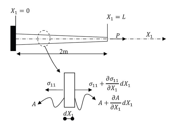
Example 2: A Bar under Axial Forces with Varying Cross Sectional Area
Let a bar with a length 2m be aligned with the coordinate axis , and let the width of the bar be equal to 250mm while the height varies linearly such that the height is equal to 500mm when  and is equal to 250mm when
  . Assume that the bar has a constant force of value 200N applied at the end
  and that the bar is fixed at the end . Find the displacement of the bar by directly solving the differential equation of equilibrium and then using the Rayleigh Ritz method assuming a polynomials of the degrees (0, 1, 2 and 3). Assume the bar to be linear elastic with Young’s modulus
  and assume that the small strain tensor is the appropriate measure of strain. Ignore the effect of Poisson’s ratio. Compare the solution obtained using the Rayleigh Ritz method with the exact solution.
Solution
Exact Solution:
First, the exact solution that would satisfy the equilibrium equations can be obtained. The equilibrium equation as shown in the beams under axial loading section when is constant and  is:
is:
![\[ EA\frac{\mathrm{d}^2u_1}{\mathrm{d}X_1^2}+E\frac{\mathrm{d}A}{\mathrm{d}X_1}\frac{\mathrm{d}u_1}{\mathrm{d}X_1}=0 \]](https://engcourses-uofa.ca/wp-content/ql-cache/quicklatex.com-7bff4fd5bfbf16830867d88210144e74_l3.png "Rendered by QuickLaTeX.com")
The area varies linearly with according to the equation:
![\[ A=0.25\left(0.5-\frac{0.25}{2}X_1\right) \]](https://engcourses-uofa.ca/wp-content/ql-cache/quicklatex.com-2e7c2224fd5ef4659d45acf3350e95cb_l3.png "Rendered by QuickLaTeX.com")
The two boundary conditions are:
![\[\begin{split} @X_1=0 & :u_1=0\\ @X_1=L & :\sigma_{11}=E\frac{\mathrm{d}u_1}{\mathrm{d}X_1}=\frac{P}{A}\bigg|_{X_1=L} \end{split} \]](https://engcourses-uofa.ca/wp-content/ql-cache/quicklatex.com-913296a8cdc6871ce9413c7a41d0b73f_l3.png "Rendered by QuickLaTeX.com")
Therefore, the exact solution for the displacement and the stress are:
![\[\begin{split} u_1 & =\frac{8}{125}\left(\ln{4}-\ln\left(4-X_1\right)\right)\\ \sigma_{11} & =\frac{6400}{4-X_1} \end{split} \]](https://engcourses-uofa.ca/wp-content/ql-cache/quicklatex.com-32d5c4ecebd4f8ecdfde62e77cb50dfc_l3.png "Rendered by QuickLaTeX.com")
Note that the exact solution for the stress could have been directly obtained by dividing the force by the variable cross sectional area. The displacement function would then be obtained by integrating the expression  .
.
View Mathematica Code
Clear[u,x]
Ax=25/100(5/10-25/200*x);
Ee=100000;
L=2;
P=200;
s=DSolve[{Ee*u''[x]*Ax+Ee*u'[x]*D[Ax,x]==0,u'[L]==200/Ee/(Ax/.x->L),u[0]==0},u,x]
u=u[x]/.s[[1]]
stress=Ee*D[u,x]
The Rayleigh Ritz Method:
The first step in the Rayleigh Ritz method finds the minimizer of the potential energy of the system which can be written as:
![\[ PE=\int\!\overline{U}\,dX - W=\int_0^L\!\frac{\sigma_{11}\varepsilon_{11}}{2}A \,\mathrm{d}X_1 - Pu_1|_{X_1=L} \]](https://engcourses-uofa.ca/wp-content/ql-cache/quicklatex.com-9a34ff9a5bf706166e97b77db6bfb97e_l3.png "Rendered by QuickLaTeX.com")
Notice that the potential energy lost by the action of the end force is equal to the product of and the displacement evaluated at . Further, we will use the constitutive equation to rewrite the potential energy function in terms of the function :
![\[ PE=\int_0^L\!\frac{EA}{2}\left(\frac{\mathrm{d}u_1}{\mathrm{d}X_1}\right)^2 \,\mathrm{d}X_1 - Pu_1|_{X_1=L} \]](https://engcourses-uofa.ca/wp-content/ql-cache/quicklatex.com-dbad5b0f8fbe41ed4dc092d1d3adf223_l3.png "Rendered by QuickLaTeX.com")
To find an approximate solution, an assumption for the shape or the form of has to be introduced. Similar to the previous example, a polynomial of the zero degree cannot be used as it will automatically render the displacement  .
.
Polynomial of the First Degree:
As a more refined approximation, we can assume that is a linear function (a polynomial of the first degree):
To satisfy the essential boundary condition the coefficient is equal to zero. Therefore:
The strain component can be computed as follows:
Substituting into the equation for the potential energy of the system:
![\[ PE=\int_0^L\!\frac{EA}{2}a_1^2 \,\mathrm{d}X_1 - Pa_1L=0.125Ea_1^2\int_0^L\!(0.5-0.125X_1) \,\mathrm{d}X_1-Pa_1L \]](https://engcourses-uofa.ca/wp-content/ql-cache/quicklatex.com-0c885802fb8c84099b06f318ef929ef5_l3.png "Rendered by QuickLaTeX.com")
The only variable that can be controlled to minimize the potential energy of the system is . Therefore:
![\[ \frac{\mathrm{d}PE}{\mathrm{d}a_1}=0\Rightarrow 18750a_1=400 \]](https://engcourses-uofa.ca/wp-content/ql-cache/quicklatex.com-2191fced3a52869b77d47b82c67cbd45_l3.png "Rendered by QuickLaTeX.com")
Therefore, the best linear function (units of m) according to the Rayleigh Ritz method is:
![\[ u_1=\frac{8}{375}X_1 \]](https://engcourses-uofa.ca/wp-content/ql-cache/quicklatex.com-a47dfaa86c45ad66f4dd3a6d9b20713f_l3.png "Rendered by QuickLaTeX.com")
A linear displacement would produce a constant stress (units of  ):
):
![\[ \sigma_{11}=\frac{6400}{3} \]](https://engcourses-uofa.ca/wp-content/ql-cache/quicklatex.com-c8e1b58c88d0ac93a808b4ed73d7003c_l3.png "Rendered by QuickLaTeX.com")
Unfortunately, this solution is far from being accurate, since it does not satisfy the differential equation of equilibrium (Why?). However, within the only possible or allowed linear shapes, the obtained solution is the minimizer of the potential energy.
Polynomial of the Second Degree:
As a more refined approximation, we can assume that is a polynomial of the second degree:
To satisfy the essential boundary condition the coefficient is equal to zero. Therefore:
The strain component can be computed as follows:
Substituting into the equation for the potential energy of the system:
![\[\begin{split} PE&=\int_0^L\!\frac{EA}{2}(a_1+2a_2X_1)^2 \,\mathrm{d}X_1 - P(a_1L+a_2L^2)\\ & = 9375a_1^2+\frac{100000}{3}a_1a_2+\frac{125000}{3}a_2^2-200(2a_1+4a_2) \end{split} \]](https://engcourses-uofa.ca/wp-content/ql-cache/quicklatex.com-d2db8f6b8e96eb572d4fab98f8a0abe7_l3.png "Rendered by QuickLaTeX.com")
and are the variables that can be controlled to minimize the potential energy of the system. Therefore:
![\[ \frac{\partial PE}{\partial a_1}=0\Rightarrow -400+18750a_1+\frac{100000}{3}a_2=0 \]](https://engcourses-uofa.ca/wp-content/ql-cache/quicklatex.com-0ab2cfaa3e0cd2b32145f207a20f6634_l3.png "Rendered by QuickLaTeX.com")
and
![\[ \frac{\partial PE}{\partial a_2}=0\Rightarrow -800+\frac{100000}{3}a_1+\frac{250000}{3}a_2=0 \]](https://engcourses-uofa.ca/wp-content/ql-cache/quicklatex.com-b47d1f6125e08892b38b19ccbfa49127_l3.png "Rendered by QuickLaTeX.com")
Solving the above two equations yields:
![\[ a_1=\frac{24}{1625}\qquad a_2=\frac{6}{1625} \]](https://engcourses-uofa.ca/wp-content/ql-cache/quicklatex.com-6fdb3adb5ed90776d63a7156145ff108_l3.png "Rendered by QuickLaTeX.com")
Therefore, the best second degree polynomial according to the Rayleigh Ritz method is:
![\[ u_1=\frac{24}{1625}X_1+\frac{6}{1625}X_1^2 \]](https://engcourses-uofa.ca/wp-content/ql-cache/quicklatex.com-8f8731193a0599904c197b944552ba60_l3.png "Rendered by QuickLaTeX.com")
A parabolic displacement would produce a linear stress:
![\[ \sigma_{11}=\frac{9600}{13}(2+X_1) \]](https://engcourses-uofa.ca/wp-content/ql-cache/quicklatex.com-968fd9b8e83b5f68e4b7f98a8caf94cc_l3.png "Rendered by QuickLaTeX.com")
Polynomial of the Third Degree:
As a more refined approximation, we can assume that is a polynomial of the third degree:
![\[ u_1 = a_0+a_1 X_1+a_2X_1^2+a_3X_1^3 \]](https://engcourses-uofa.ca/wp-content/ql-cache/quicklatex.com-75f596a5c5c82c789272400ee12a06b1_l3.png "Rendered by QuickLaTeX.com")
To satisfy the essential boundary condition the coefficient is equal to zero. Therefore:
![\[ u_1 = a_1 X_1+a_2X_1^2+a_3X_1^3 \]](https://engcourses-uofa.ca/wp-content/ql-cache/quicklatex.com-449eb712d2774561a290678461c9c07a_l3.png "Rendered by QuickLaTeX.com")
The strain component can be computed as follows:
![\[ \varepsilon_{11}=\frac{\mathrm{d}u_1}{\mathrm{d}X_1}=a_1+2a_2X_1+3a_3X_1^2 \]](https://engcourses-uofa.ca/wp-content/ql-cache/quicklatex.com-ac554b855d35da73cc9afcb1dbde3ad1_l3.png "Rendered by QuickLaTeX.com")
Substituting into the equation for the potential energy of the system:
![\[\begin{split} PE&=\int_0^L\!\frac{EA}{2}(a_1+2a_2X_1+3a_3X_1^2)^2 \,\mathrm{d}X_1 - P(a_1L+a_2L^2+a_3L^3)\\ & = 9375a_1^2+\frac{100000}{3}a_1a_2+\frac{125000}{3}a_2^2+62500a_1a_3+180000a_2a_3+210000a_3^2\\ &-200(2a_1+4a_2+8a_3) \end{split} \]](https://engcourses-uofa.ca/wp-content/ql-cache/quicklatex.com-ebda41c27cc83cdf8f8d48452b9a54b6_l3.png "Rendered by QuickLaTeX.com")
, , and are the variables that can be controlled to minimize the potential energy of the system. Therefore:
![\[ \frac{\partial PE}{\partial a_1}=0\Rightarrow -400+18750a_1+\frac{100000}{3}a_2+62500a_3=0 \]](https://engcourses-uofa.ca/wp-content/ql-cache/quicklatex.com-37addf9373918a6354aa6843d546a17e_l3.png "Rendered by QuickLaTeX.com")
Also:
![\[ \frac{\partial PE}{\partial a_2}=0\Rightarrow -800+\frac{100000}{3}a_1+\frac{250000}{3}a_2+180000a_3=0 \]](https://engcourses-uofa.ca/wp-content/ql-cache/quicklatex.com-7220cfdfbd362ee10df4f10e61bd5107_l3.png "Rendered by QuickLaTeX.com")
And:
![\[ \frac{\partial PE}{\partial a_3}=0\Rightarrow -1600+62500a_1+180000a_2+420000a_3=0 \]](https://engcourses-uofa.ca/wp-content/ql-cache/quicklatex.com-051847527343761c0136ccfbf85fa662_l3.png "Rendered by QuickLaTeX.com")
Solving the above three equations yields:
![\[ a_1=\frac{128}{7875}\qquad a_2=\frac{2}{1575} \qquad a_3=\frac{4}{4725} \]](https://engcourses-uofa.ca/wp-content/ql-cache/quicklatex.com-ea33e3dbf90eae3d89a297d8c72086d4_l3.png "Rendered by QuickLaTeX.com")
Therefore, the best third degree polynomial according to the Rayleigh Ritz method is:
![\[ u_1=\frac{128}{7875}X_1+\frac{2}{1575}X_1^2+\frac{4}{4725}X_1^3 \]](https://engcourses-uofa.ca/wp-content/ql-cache/quicklatex.com-32baa6e1051e1c0665bc856f64b0d460_l3.png "Rendered by QuickLaTeX.com")
A cubic displacement would produce a parabolic stress distribution:
![\[ \sigma_{11}=\frac{3200}{63}(32+5X_1(1+X_1)) \]](https://engcourses-uofa.ca/wp-content/ql-cache/quicklatex.com-7e02c62ead73d080119c726b0dcb0e27_l3.png "Rendered by QuickLaTeX.com")
Clear[u, u1, u2, u3, u4, stress, stress1, stress2, stress3, x]
(*Exact Solution *)
Ax=25/100(5/10-25/200*x);
Ee=100000;
L=2;
P=200;
s=DSolve[{Ee*u''[x]*Ax+Ee*u'[x]*D[Ax,x]==0,u'[L]==200/Ee/(Ax/.x->L),u[0]==0},u,x]
u=u[x]/.s[[1]];
stress=Ee*D[u,x]
(*First Degree *)
u1=a1*x;
PE=Integrate[1/2*Ee*D[u1,x]^2*Ax,{x,0,L}]-P*u1/.x->L;
Eq1=D[PE,a1];
s=Solve[Eq1==0,a1];
u1=u1/.s[[1]];
stress1=Ee*D[u1,x];
(*Second Degree *)
u2=a1*x+a2*x^2;
PE=Integrate[1/2*Ee*D[u2,x]^2*Ax,{x,0,L}]-P*u2/.x-> L;
Eq1=D[PE,a1];
Eq2=D[PE,a2];
s=Solve[{Eq1==0,Eq2==0},{a1,a2}];
u2=u2/.s[[1]];
stress2=Ee*D[u2,x];
(*Third Degree *)
u3=a1*x+a2*x^2+a3*x^3;
PE=Integrate[1/2*Ee*D[u3,x]^2*Ax,{x,0,L}]-P*u3/.x->L;
Eq1=D[PE,a1];
Eq2=D[PE,a2];
Eq3=D[PE,a3];
s=Solve[{Eq1==0,Eq2==0,Eq3==0},{a1,a2,a3}];
u3=u3/.s[[1]];
stress3=Ee*D[u3,x];
(*comparison*)
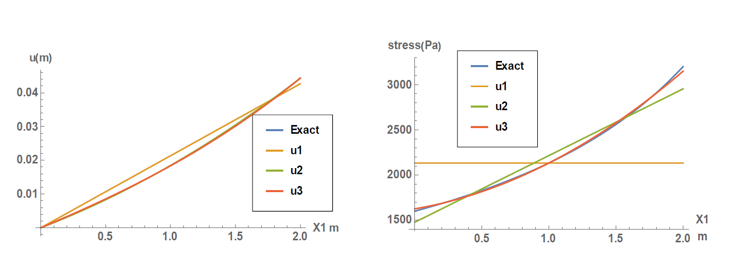
Plot[{u, u1, u2, u3}, {x, 0, L}, PlotLegends -> {Style["Exact", Bold, 12], Style["u1", Bold, 12], Style["u2", Bold, 12], Style["u3", Bold, 12]}, AxesLabel -> {"X1 m", "u(m)"}, BaseStyle -> Directive[Bold, 12]]
Plot[{stress, stress1, stress2, stress3}, {x, 0, L}, AxesLabel -> {"X1 m", "stress(Pa)"}, BaseStyle -> Directive[Bold, 12], PlotLegends -> {Style["Exact", Bold, 12], Style["u1", Bold, 12], Style["u2", Bold, 12], Style["u3", Bold, 12]}]
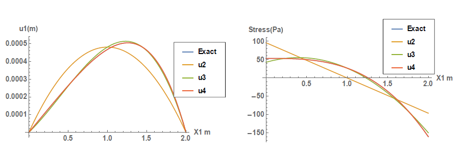
The exact solution obtained is a logarithmic function, while the approximations used for the Rayleigh Ritz method are polynomial functions. The Taylor series of a logarithmic function can be represented by a linear combination of polynomial functions, and so, the higher the degree of approximation, the closer the approximation to the exact solution. As seen in the plots below, good accuracy is obtained for a polynomial of the second degree for the displacement function; however, the stresses in that case have higher errors. A better approximation for the stresses is obtained using a polynomial of the third degree. In general, the error in the approximate solution (i.e., the error in ) is less than the error in its derivatives which in this case is the value of the strain component . This means as well that in order to achieve higher accuracy in the stress , higher polynomials are needed.
Example 3: A Bar under Varying Body Forces with Fixed Ends
Let a bar with a length 2mbe aligned with the coordinate axis , and let the cross sectional area of the bar be equal to  . Assume that the bar is fixed at both ends
  and . Assume that the bar is subjected to a varying body force that is equal to
  in the direction of the coordinate axis . Find the displacement of the bar by directly solving the differential equation of equilibrium and then using the Rayleigh Ritz method assuming polynomials of the degrees (0, 1, 2, 3, and 4). Assume that the bar material is linear elastic with Young’s modulus
  and that the small strain tensor is the appropriate measure of strain. Ignore the effect of Poisson’s ratio. Compare the solution obtained using the Rayleigh Ritz method using three- and four-degree polynomials as approximations with the exact solution.

Solution
Exact Solution:
Similar to the previous examples, the equilibrium equation is:
![\[ \frac{\mathrm{d}^2u_1}{\mathrm{d}X_1^2}=-\frac{p}{EA}=-\frac{5X_1^2}{0.25^2E} \]](https://engcourses-uofa.ca/wp-content/ql-cache/quicklatex.com-0d551479e48f79cf4a8acab57df37f9f_l3.png "Rendered by QuickLaTeX.com")
Therefore, the solution for has the form:
![\[ u_1=-\frac{5X_1^4}{12(0.25)^2E}+C_1X_1+C_2 \]](https://engcourses-uofa.ca/wp-content/ql-cache/quicklatex.com-4cd57199cbfea49bf036b427211acb73_l3.png "Rendered by QuickLaTeX.com")
The boundary conditions for this example are:
![\[\begin{split} @X_1=0&:u_1=0\Rightarrow C_2=0\\ @X_1=L&:u_1=0\Rightarrow C_1=\frac{5L^3}{12(0.25)^2E} \end{split} \]](https://engcourses-uofa.ca/wp-content/ql-cache/quicklatex.com-0043ab1203f15b44064e47982dd815b3_l3.png "Rendered by QuickLaTeX.com")
Therefore the exact solutions for the displacement (in m) and the stress (in ) are:
![\[\begin{split} u_1&=\frac{8X_1-X_1^4}{15000}\\ \sigma_{11}&=\frac{20}{3}(8-4X_1^3) \end{split} \]](https://engcourses-uofa.ca/wp-content/ql-cache/quicklatex.com-8c58ea2aa9f9a96dafdebf3cd5e4b5d5_l3.png "Rendered by QuickLaTeX.com")
The Rayleigh Ritz Method:
The first step in the Rayleigh Ritz method finds the minimizer of the potential energy of the system which can be written as:
![\[ PE=\int\!\overline{U}\,dX - W=\int_0^L\!\frac{\sigma_{11}\varepsilon_{11}}{2}A \,\mathrm{d}X_1 - \int_0^L\!pu_1\,\mathrm{d}X_1 \]](https://engcourses-uofa.ca/wp-content/ql-cache/quicklatex.com-eac0eb030a2b04c346a3a1dbfb4a8005_l3.png "Rendered by QuickLaTeX.com")
Notice that the potential energy lost by the action of the distributed body forces is an integral since it acts on each point along the beam length. Further, we will use the constitutive equation to rewrite the potential energy function in terms of the function :
![\[ PE=\int_0^L\!\frac{EA}{2}\left(\frac{\mathrm{d}u_1}{\mathrm{d}X_1}\right)^2 \,\mathrm{d}X_1 - \int_0^L\!5X_1^2u_1\,\mathrm{d}X_1 \]](https://engcourses-uofa.ca/wp-content/ql-cache/quicklatex.com-cbb8d22319cbfe88a49c7715db1ad091_l3.png "Rendered by QuickLaTeX.com")
To find an approximate solution, an assumption for the shape or the form of has to be introduced.
Polynomials of the Zero and First Degrees:
Assuming that that is a constant function (a polynomial of the zero degree) or a linear function (a polynomial of the first degree) and incorporating the boundary conditions:
![\[\begin{split} @X_1=0&:u_1=0\\ @X_1=L&:u_1=0 \end{split} \]](https://engcourses-uofa.ca/wp-content/ql-cache/quicklatex.com-a43e625ac8f2aad5bb70b9057298ea96_l3.png "Rendered by QuickLaTeX.com")
leads to the trivial solution , which will automatically be rejected.
Polynomial of the Second Degree:
Let be a polynomial of the second degree:
The essential boundary condition can be used to find values for the constants and as follows:
![\[\begin{split} @X_1=0&:u_1=0\Rightarrow a_0=0\\ @X_1=L&:u_1=0\Rightarrow a_2=-\frac{a_1}{L} \end{split} \]](https://engcourses-uofa.ca/wp-content/ql-cache/quicklatex.com-09dee747fc35d0a4793b5ce4731c82ed_l3.png "Rendered by QuickLaTeX.com")
Therefore, the displacement function has only one parameter that can be controlled:
![\[ u_1=a_1X_1\left(1-\frac{X_1}{L}\right) \]](https://engcourses-uofa.ca/wp-content/ql-cache/quicklatex.com-e509c9ea0ccdc3c6e6c1551f76c0ed11_l3.png "Rendered by QuickLaTeX.com")
The strain component can be computed as follows:
![\[ \varepsilon_{11}=\frac{\mathrm{d}u_1}{\mathrm{d}X_1}=a_1\left(1-2\frac{X_1}{L}\right) \]](https://engcourses-uofa.ca/wp-content/ql-cache/quicklatex.com-4a355556746dbfd746335eff71a717a6_l3.png "Rendered by QuickLaTeX.com")
Substituting into the equation for the potential energy of the system:
![\[\begin{split} PE&=\int_0^L\!\frac{EA}{2}\left(a_1\left(1-2\frac{X_1}{L}\right)\right)^2 \,\mathrm{d}X_1 -\int_0^L\!5X_1^2a_1X_1\left(1-\frac{X_1}{L}\right)\,\mathrm{d}X_1\\ & = \frac{6250}{3}a_1^2-4a_1 \end{split} \]](https://engcourses-uofa.ca/wp-content/ql-cache/quicklatex.com-745cf6bc9ea9ccdbe661b78450e9053a_l3.png "Rendered by QuickLaTeX.com")
can be found by minimizing the potential energy of the system. Therefore:
![\[ \frac{\mathrm{d}PE}{\mathrm{d}a_1}=0\Rightarrow \frac{12500}{3}a_1-4=0\Rightarrow a_1=\frac{3}{3125} \]](https://engcourses-uofa.ca/wp-content/ql-cache/quicklatex.com-2129b49333de2b48f43d2ef98d58857d_l3.png "Rendered by QuickLaTeX.com")
Therefore, the best second degree polynomial according to the Rayleigh Ritz method is:
![\[ u_1=\frac{3X_1}{3125}\left(1-\frac{X_1}{2}\right) \]](https://engcourses-uofa.ca/wp-content/ql-cache/quicklatex.com-2fb3ef51b0e614c7a253381c4bc266ae_l3.png "Rendered by QuickLaTeX.com")
A parabolic displacement would produce a linear stress:
![\[ \sigma_{11}=96(1-X_1) \]](https://engcourses-uofa.ca/wp-content/ql-cache/quicklatex.com-1e6e2f17adc584d5c7d7dda5a6f8fe98_l3.png "Rendered by QuickLaTeX.com")
Polynomials of Higher Degrees:
The results from the following Mathematica code show that the third-degree approximation is very close to the actual solution for both displacements and stresses. The polynomial of the
fourth-degree approximation is in fact exact since the exact solution is a polynomial of the fourth degree. Study the Mathematica code carefully to understand how the second boundary conditions of displacement are incorporated. The graph comparing the results are shown below.
Clear[u, x, a1, a2, a3, a4, a5, a0, Ee, A, L, p, u3, u4]
p = 5 x^2;
s = DSolve[{Ee*u''[x] == -p/A, u[L] == 0, u[0] == 0}, u, x];
u = u[x] /. s[[1]];
stress = Ee*D[u, x];
(*Second Degree*)
u2 = a2*x^2 + a1*x;
sol = Solve[(u2 /. x -> L) == 0, a2];
u2 = u2 /. sol[[1]];
PE = 1/2*Integrate[Ee*A*D[u2, x]^2, {x, 0, L}] - Integrate[p*u2, {x, 0, L}];
Eq1 = D[PE, a1];
sol1 = Solve[{Eq1 == 0}, {a1}];
u2 = FullSimplify[u2 /. sol1[[1]]];
stress2 = FullSimplify[Ee*D[u2, x]];
(*Third Degree*)
u3 = a3*x^3 + a2*x^2 + a1*x;
sol = Solve[(u3 /. x -> L) == 0, a3];
u3 = u3 /. sol[[1]];
PE = 1/2*Integrate[Ee*A*D[u3, x]^2, {x, 0, L}] -  Integrate[p*u3, {x, 0, L}];
Eq1 = D[PE, a1];
Eq2 = D[PE, a2];
sol1 = Solve[{Eq1 == 0, Eq2 == 0}, {a2, a1}];
u3 = FullSimplify[u3 /. sol1[[1]]];
stress3 = FullSimplify[Ee*D[u3, x]];
(*Fourth Degree*)
u4 = a4*x^4 + a3*x^3 + a2*x^2 + a1*x;
sol = Solve[(u4 /. x -> L) == 0, a4];
u4 = u4 /. sol[[1]];
PE = 1/2*Integrate[Ee*A*D[u4, x]^2, {x, 0, L}] -   Integrate[p*u4, {x, 0, L}];
Eq1 = D[PE, a1];
Eq2 = D[PE, a2];
Eq3 = D[PE, a3];
sol1 = Solve[{Eq1 == 0, Eq2 == 0, Eq3 == 0}, {a1, a2, a3}];
u4 = FullSimplify[u4 /. sol1[[1]]];
stress4 = FullSimplify[Ee*D[u4, x]];
A = (25/100)^2;
Ee = 100000;
L = 2;
(*comparison*)
Plot[{u, u2, u3, u4}, {x, 0, L},  PlotLegends -> {Style["Exact", Bold, 12], Style["u2", Bold, 12],    Style["u3", Bold, 12], Style["u4", Bold, 12]},  AxesLabel -> {"X1 m", "u1(m)"}, BaseStyle -> Directive[Bold, 12]]
Plot[{stress, stress2, stress3, stress4}, {x, 0, L},  PlotLegends -> {Style["Exact", Bold, 12], Style["u2", Bold, 12],    Style["u3", Bold, 12], Style["u4", Bold, 12]},  AxesLabel -> {"X1 m", "Stress(Pa)"},  BaseStyle -> Directive[Bold, 12]]
Euler Bernoulli Beams under Lateral Loading
For plane Euler Bernoulli beams under lateral loading, the unknown displacement function is  . In this case, the potential energy of the system has the following form (See Euler Bernoulli Beam and energy expressions):
![\[ PE=\mbox{Total Strain Energy} - W=\int\!\frac{EI}{2}\left(\frac{\mathrm{d}^2y}{\mathrm{d}X_1^2}\right)^2 \,\mathrm{d}X_1 - W \]](https://engcourses-uofa.ca/wp-content/ql-cache/quicklatex.com-fb40d41b53d143e4356c69c11f4a7375_l3.png "Rendered by QuickLaTeX.com")
where is Young’s modulus,  is the moment of inertia, and is the work done by all the external forces acting on the bar (concentrated forces and distributed loads). A few examples to solve for the displacements, rotations, shear forces, and moments for an Euler Bernoulli beam under lateral loading are presented in this section. Similar to the previous section, the Rayleigh Ritz method starts by choosing a form for the displacement function. This form has to satisfy the “essential” boundary conditions, which for this particular type of problems are those boundary conditions imposed on the displacements and the rotations. The following examples show the method for different external loads, and beam configurations.
Example 1: Cantilever Beam
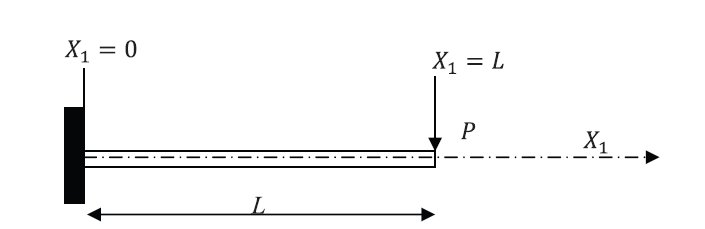
Let a beam with a length and a constant cross sectional parameters area and moment of inertia be aligned with the coordinate axis . Assume that the beam is subjected to a constant force of value applied at the end  in the direction shown in the figure. Assume that the bar is fixed (rotation and displacement are equal to zero) at the end . Find the displacement, rotation, bending moment, and shearing forces on the beam by directly solving the differential equation of equilibrium and then using the Rayleigh Ritz method assuming polynomials of the degrees (0,1, 2, 3, and 4). Assume the beam to be linear elastic with Young’s modulus and that the Euler Bernoulli Beam is an appropriate beam approximation.
Solution
Exact Solution:
First, the exact solution that would satisfy the equilibrium equations can be obtained. The equilibrium equation as shown in the Euler Bernoulli beam section when and are constant is:
![\[ EI\frac{\mathrm{d}^4y}{\mathrm{d}X_1^4}=q \]](https://engcourses-uofa.ca/wp-content/ql-cache/quicklatex.com-61329386e1995043b92c53b4b10a55bf_l3.png "Rendered by QuickLaTeX.com")
For the shown cantilever beam,  and therefore the exact solution for the displacement has the form:
![\[ y=\frac{C_1X_1^3}{6}+\frac{C_2X_1^2}{2}+C_3X_1+C_4 \]](https://engcourses-uofa.ca/wp-content/ql-cache/quicklatex.com-df1c00ab12c95bd3a4ad00913253b376_l3.png "Rendered by QuickLaTeX.com")
where the constants can be obtained from the boundary conditions:
![\[ \begin{split} & @X_1=0:y=0\Rightarrow C_4=0\\ & @X_1=0:\theta=\frac{\mathrm{d}y}{\mathrm{d}X_1}=0\Rightarrow C_3=0\\ & @X_1=L:M=0\Rightarrow EI\frac{\mathrm{d}^2y}{\mathrm{d}X_1^2}=0\Rightarrow C_2=-C_1L\\ & @X_1=L:V=P\Rightarrow EI\frac{\mathrm{d}^3y}{\mathrm{d}X_1^3}=P\Rightarrow C_1=\frac{P}{EI} \end{split} \]](https://engcourses-uofa.ca/wp-content/ql-cache/quicklatex.com-e12f5a0811940098cd72163c9f128106_l3.png "Rendered by QuickLaTeX.com")
Therefore, the exact solution for the displacement , the rotation  , the moment
  , and the shear are:
![\[\begin{split} y & =\frac{PX_1^3}{6EI}-\frac{PLX_1^2}{2EI}\\ \theta & = \frac{\mathrm{d}y}{\mathrm{d}X_1}=\frac{PX_1^2}{2EI}-\frac{PLX_1}{EI}\\ M & = EI\frac{\mathrm{d}^2y}{\mathrm{d}X_1^2}=PX_1-PL\\ V & = EI\frac{\mathrm{d}^3y}{\mathrm{d}X_1^3}=P \end{split} \]](https://engcourses-uofa.ca/wp-content/ql-cache/quicklatex.com-ca1bd560560d122530324c689a493906_l3.png "Rendered by QuickLaTeX.com")
The Rayleigh Ritz Method:
The first step in the Rayleigh Ritz method finds the minimizer of the potential energy of the system which can be written as:
![\[ PE=\int\!\overline{U}\,dX - W=\int_0^L\!\frac{EI}{2}\left(\frac{\mathrm{d}^2y}{\mathrm{d}X_1^2}\right)^2 \,\mathrm{d}X_1 - (-P)y|_{X_1=L} \]](https://engcourses-uofa.ca/wp-content/ql-cache/quicklatex.com-5241ce0c9682381940951cdf6885c758_l3.png "Rendered by QuickLaTeX.com")
Notice that the potential energy lost by the action of the end force is equal to the product of  ( is acting downwards and is assumed upwards) and the displacement evaluated at . To find an approximate solution, an assumption for the shape or the form of has to be introduced.
Polynomials of the Zero and First Degrees:
If we assume that is a constant (polynomial of the zero degree) or a linear (polynomial of the first degree) function, and when attempting to satisfy the essential boundary conditions:
![\[\begin{split} @X_1=0 & :y=0\\ @X_1=0 & :\theta=\frac{\mathrm{d}y}{\mathrm{d}X_1}=0 \end{split} \]](https://engcourses-uofa.ca/wp-content/ql-cache/quicklatex.com-32628f417c0250082b65e9730c95d18a_l3.png "Rendered by QuickLaTeX.com")
this leads to the trivial solution  , which will automatically be rejected.
Polynomial of the Second Degree:
The approximate solution forms for the displacement , the rotation , the moment , and the shear force functions if is assumed to be a polynomial of the second degree are:
![\[ \begin{split} y & =a_2X_1^2+a_1X_1+a_0\\ \theta &=\frac{\mathrm{d}y}{\mathrm{d}X_1} =2a_2X_1+a_1\\ M &=EI\frac{\mathrm{d}^2y}{\mathrm{d}X_1^2} =2EIa_2\\ V &=0 \end{split} \]](https://engcourses-uofa.ca/wp-content/ql-cache/quicklatex.com-54e323ada49557380922d5022e73f9ba_l3.png "Rendered by QuickLaTeX.com")
To satisfy the essential boundary conditions, we have:
![\[ \begin{split} @X_1=0 & :y=0\Rightarrow a_0=0\\ @X_1=0 & :\theta=\frac{\mathrm{d}y}{\mathrm{d}X_1}=0\Rightarrow a_1=0 \end{split} \]](https://engcourses-uofa.ca/wp-content/ql-cache/quicklatex.com-cb09bafc935bbb534611c7fbcb8acc6d_l3.png "Rendered by QuickLaTeX.com")
Therefore, the solutions forms have only one parameter that can be controlled:
![\[ \begin{split} y & =a_2X_1^2\\ \theta &=\frac{\mathrm{d}y}{\mathrm{d}X_1} =2a_2X_1\\ M &=EI\frac{\mathrm{d}^2y}{\mathrm{d}X_1^2} =2EIa_2\\ V &=0 \end{split} \]](https://engcourses-uofa.ca/wp-content/ql-cache/quicklatex.com-55949c158447469065b21a0127b5a7f4_l3.png "Rendered by QuickLaTeX.com")
Substituting into the equation of the potential energy of an Euler Bernoulli beam:
![\[ PE=\frac{EI}{2}\int_0^L\!\left(2a_2\right)^2\,\mathrm{d}X_1+P\left(a_2L^2\right) \]](https://engcourses-uofa.ca/wp-content/ql-cache/quicklatex.com-64ca6b380b2718b1ab192f69b04c88eb_l3.png "Rendered by QuickLaTeX.com")
The unknown coefficient can be obtained by minimizing the potential energy:
![\[ \frac{\mathrm{d} PE}{\mathrm{d} a_2} =4EILa_2+PL^2=0\Rightarrow a_2=-\frac{PL}{4EI} \]](https://engcourses-uofa.ca/wp-content/ql-cache/quicklatex.com-de2477b508289cd80a2bd4a3139041d3_l3.png "Rendered by QuickLaTeX.com")
Therefore, the “best” parabolic approximation for along with the corresponding solutions for , , and are given by:
![\[ \begin{split} y & =-\frac{PLX_1^2}{4EI}\\ \theta &=\frac{\mathrm{d}y}{\mathrm{d}X_1} =-\frac{PLX_1}{2EI}\\ M &=EI\frac{\mathrm{d}^2y}{\mathrm{d}X_1^2} =-\frac{PL}{2}\\ V &=EI\frac{\mathrm{d}^3y}{\mathrm{d}X_1^3} =0 \end{split} \]](https://engcourses-uofa.ca/wp-content/ql-cache/quicklatex.com-bc6dc9d5595541c9dcfbb48381151034_l3.png "Rendered by QuickLaTeX.com")
Note that because of the simplicity of the approximation, the shear force (which is the third derivative) is always equal to zero.
Polynomial of the Third Degree:
The approximate solution forms for the displacement , the rotation , the moment , and the shear force functions if is assumed to be a polynomial of the third degree are:
![\[ \begin{split} y & =a_3X_1^3+a_2X_1^2+a_1X_1+a_0\\ \theta &=\frac{\mathrm{d}y}{\mathrm{d}X_1} =3a_3X_1^2+2a_2X_1+a_1\\ M &=EI\frac{\mathrm{d}^2y}{\mathrm{d}X_1^2} =6EIa_3X_1+2EIa_2\\ V &=6EIa_3 \end{split} \]](https://engcourses-uofa.ca/wp-content/ql-cache/quicklatex.com-f918d99294ae040f67317fc116c26032_l3.png "Rendered by QuickLaTeX.com")
To satisfy the essential boundary conditions, we have:
Therefore, the solutions forms have only two parameters and that can be controlled:
![\[ \begin{split} y & =a_3X_1^3+a_2X_1^2\\ \theta &=\frac{\mathrm{d}y}{\mathrm{d}X_1} =3a_3X_1^2+2a_2X_1\\ M &=EI\frac{\mathrm{d}^2y}{\mathrm{d}X_1^2} =6EIa_3X_1+2EIa_2\\ V &=6EIa_3 \end{split} \]](https://engcourses-uofa.ca/wp-content/ql-cache/quicklatex.com-a54a880f7fe0480935b0ae0e2619618f_l3.png "Rendered by QuickLaTeX.com")
Substituting into the equation of the potential energy of an Euler Bernoulli beam:
![\[ PE=\frac{EI}{2}\int_0^L\!\left(6a_3X_1+2a_2\right)^2\,\mathrm{d}X_1+P\left(a_3L^3+a_2L^2\right) \]](https://engcourses-uofa.ca/wp-content/ql-cache/quicklatex.com-5474b01bdf45d6a7a5c234f178e0cace_l3.png "Rendered by QuickLaTeX.com")
The unknown coefficients and can be obtained by minimizing the potential energy:
![\[\begin{split} \frac{\partial PE}{\partial a_2} & =\frac{EI}{2}(8a_2L+12a_3L^2)+PL^2=0\\ \frac{\partial PE}{\partial a_3} & =\frac{EI}{2}(12a_2L^2+24a_3L^3)+PL^3=0 \end{split} \]](https://engcourses-uofa.ca/wp-content/ql-cache/quicklatex.com-2272719df0180132a7d764930c566de9_l3.png "Rendered by QuickLaTeX.com")
Solving the above two equations yields:
![\[ a_2=-\frac{PL}{2EI} \qquad a_3=\frac{P}{6EI} \]](https://engcourses-uofa.ca/wp-content/ql-cache/quicklatex.com-01d49f236780bdd0f432c24eb5b8a1b8_l3.png "Rendered by QuickLaTeX.com")
Therefore, the “best” cubic approximation for along with the corresponding solutions for , , and are given by:
![\[ \begin{split} y & =\frac{PX_1^3}{6EI}-\frac{PLX_1^2}{2EI}\\ \theta &=\frac{\mathrm{d}y}{\mathrm{d}X_1} =\frac{PX_1^2}{2EI}-\frac{PLX_1}{EI}\\ M &=EI\frac{\mathrm{d}^2y}{\mathrm{d}X_1^2} =PX_1-PL\\ V &=EI\frac{\mathrm{d}^3y}{\mathrm{d}X_1^3} =P \end{split} \]](https://engcourses-uofa.ca/wp-content/ql-cache/quicklatex.com-e1c4a62985c1ee85ff171523670e5917_l3.png "Rendered by QuickLaTeX.com")
The “approximate” solution obtained here is identical to the “exact” solution obtained above. This is because the trial function for was assumed to be a cubic polynomial and the exact solution is in fact a cubic polynomial. One should note that when the “form” or “shape” of the approximate solution contains the “form” or “shape” of the exact solution, then the Rayleigh Ritz method renders the exact solution! To see this, we are going to try a finer approximation (A polynomial of the fourth degree).
Polynomial of the Fourth Degree:
The approximate solution forms for the displacement , the rotation , the moment , and the shear force functions if is assumed to be a polynomial of the fourth degree are:
![\[ \begin{split} y & =a_4X_1^4+a_3X_1^3+a_2X_1^2+a_1X_1+a_0\\ \theta &=\frac{\mathrm{d}y}{\mathrm{d}X_1} =4a_4X_1^3+3a_3X_1^2+2a_2X_1+a_1\\ M &=EI\frac{\mathrm{d}^2y}{\mathrm{d}X_1^2} =12EIa_4X_1^2+6EIa_3X_1+2EIa_2\\ V &=24EIa_4X_1+6EIa_3 \end{split} \]](https://engcourses-uofa.ca/wp-content/ql-cache/quicklatex.com-a92e34c557ffe4232b32ac77a6e9c2da_l3.png "Rendered by QuickLaTeX.com")
To satisfy the essential boundary conditions, we have:
Therefore, the solutions forms have the parameters , , and  that can be controlled:
![\[ \begin{split} y & =a_4X_1^4+a_3X_1^3+a_2X_1^2\\ \theta &=\frac{\mathrm{d}y}{\mathrm{d}X_1} =4a_4X_1^3+3a_3X_1^2+2a_2X_1\\ M &=EI\frac{\mathrm{d}^2y}{\mathrm{d}X_1^2} =12EIa_4X_1^2+6EIa_3X_1+2EIa_2\\ V &=24EIa_4X_1+6EIa_3 \end{split} \]](https://engcourses-uofa.ca/wp-content/ql-cache/quicklatex.com-3d128e1a7289964220168028a88acb11_l3.png "Rendered by QuickLaTeX.com")
Substituting into the equation of the potential energy of an Euler Bernoulli beam:
![\[ PE=\frac{EI}{2}\int_0^L\!\left(12a_4X_1^2+6a_3X_1+2a_2\right)^2\,\mathrm{d}X_1+P\left(a_4L^4+a_3L^3+a_2L^2\right) \]](https://engcourses-uofa.ca/wp-content/ql-cache/quicklatex.com-f784f07b6c0bb3554731ef49c1e48dab_l3.png "Rendered by QuickLaTeX.com")
The unknown coefficients , , and can be obtained by minimizing the potential energy:
![\[ \frac{\partial PE}{\partial a_2} =0\qquad \frac{\partial PE}{\partial a_3} =0 \qquad \frac{\partial PE}{\partial a_4} =0 \]](https://engcourses-uofa.ca/wp-content/ql-cache/quicklatex.com-9cd884289a030283f25face5538e8b94_l3.png "Rendered by QuickLaTeX.com")
Solving the above three equations yields:
![\[ a_2=-\frac{PL}{2EI} \qquad a_3=\frac{P}{6EI} \qquad a_4=0 \]](https://engcourses-uofa.ca/wp-content/ql-cache/quicklatex.com-22f16ce8be2be16910175f71bb05897a_l3.png "Rendered by QuickLaTeX.com")
Therefore, assuming a fourth order polynomial gives the same solution as a third order polynomial!
View Mathematica Code(*Exact Solution*)
Clear[a,x,V,M,P,y,L,EI]
M=EI*D[y[x],{x,2}];
V=EI*D[y[x],{x,3}];
th=D[y[x],x];
q=0;
M1=M/.x->0;
M2=M/.x->L;
V1=V/.x->0;
V2=V/.x->L;
y1=y[x]/.x->0;
y2=y[x]/.x->L;
th1=th/.x->0;
th2=th/.x->L;
s=DSolve[{EI*y''''[x]==q,y1==0,th1==0,V2==P,M2==0},y,x];
y=y[x]/.s[[1]]
th=D[y,x]
M=EI*D[y,{x,2}]
V=EI*D[y,{x,3}]
(*Second Degree*)
Clear[y,x,M,V,th,EI,PE]
y=a2*x^2
th=D[y,x];
M=EI*D[y,{x,2}];
V=EI*D[y,{x,3}];
PE=EI/2*Integrate[D[y,{x,2}]^2,{x,0,L}]+P*(y/.x->L);
Eq2=D[PE,a2];
Sol=Solve[{Eq2==0},{a2}]
y=y/.Sol[[1]]
th/.Sol[[1]]
FullSimplify[M/.Sol[[1]]]
FullSimplify[V/.Sol[[1]]]
(*Third Degree*)
Clear[y,x,M,V,th,EI,PE]
y=a3*x^3+a2*x^2
th=D[y,x];
M=EI*D[y,{x,2}];
V=EI*D[y,{x,3}];
PE=EI/2*Integrate[D[y,{x,2}]^2,{x,0,L}]+P*(y/.x->L);
Eq1=D[PE,a3];
Eq2=D[PE,a2];
Sol=Solve[{Eq1==0,Eq2==0},{a3,a2}]
y=y/.Sol[[1]]
th/.Sol[[1]]
FullSimplify[M/.Sol[[1]]]
FullSimplify[V/.Sol[[1]]]
(*Fourth Degree*)
Clear[y,x,M,V,th,EI,PE]
y=a4*x^4+a3*x^3+a2*x^2
th=D[y,x];
M=EI*D[y,{x,2}];
V=EI*D[y,{x,3}];
PE=EI/2*Integrate[D[y,{x,2}]^2,{x,0,L}]+P*(y/.x->L);
Eq1=D[PE,a3];
Eq2=D[PE,a2];
Eq3=D[PE,a4];
Sol=Solve[{Eq1==0,Eq2==0,Eq3==0},{a3,a2,a4}]
y=y/.Sol[[1]]
th/.Sol[[1]]
FullSimplify[M/.Sol[[1]]]
FullSimplify[V/.Sol[[1]]]
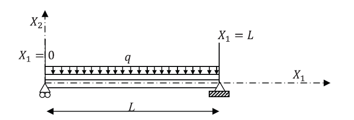
Example 2: Simple Beam
Let a beam with a length  and a constant moment of inertia
  be aligned with the coordinate axis . Assume that the beam is subjected to a distributed load
  .(Notice that the negative sign was added since
  is positive when it is in the direction of positive
  ). Assume that the beam is hinged at the ends and . Find the displacement, rotation, bending moment, and shearing forces on the beam by directly solving the differential equation of equilibrium and then using the Rayleigh Ritz method assuming polynomials of the degrees (0, 1, 2, 3 and 4). Assume the beam to be linear elastic with Young’s modulus
  and that the Euler Bernoulli Beam is an appropriate beam approximation. Compare the Rayleigh Ritz method with the exact solution.
Solution
Exact Solution:
First, the exact solution that would satisfy the equilibrium equations can be obtained. The equilibrium equation as shown in the Euler Bernoulli beam section when and are constant is:
For the shown simple beam,  and therefore the exact solution for the displacement has the form:
![\[ y=q\frac{X_1^4}{24}+\frac{C_1X_1^3}{6}+\frac{C_2X_1^2}{2}+C_3X_1+C_4 \]](https://engcourses-uofa.ca/wp-content/ql-cache/quicklatex.com-77cb581231af332922e1138579561fb3_l3.png "Rendered by QuickLaTeX.com")
where the constants can be obtained from the boundary conditions:
![\[ \begin{split} & @X_1=0:y=0\Rightarrow C_4=0\\ & @X_1=0:M=EI\frac{\mathrm{d}^2y}{\mathrm{d}X_1^2}=0\Rightarrow C_2=0\\ & @X_1=L:y=0\Rightarrow q\frac{L^4}{24}+\frac{C_1L^3}{6}+C_3L=0\\ & @X_1=L:M=EI\frac{\mathrm{d}^2y}{\mathrm{d}X_1^2}=0\Rightarrow q\frac{L^2}{2}+C_1L=0\\ \end{split} \]](https://engcourses-uofa.ca/wp-content/ql-cache/quicklatex.com-c0152fda9d7f8ab90de0dd2059ab49c9_l3.png "Rendered by QuickLaTeX.com")
therefore,
![\[ C_1=-\frac{qL}{2}\qquad C_3=\frac{qL^3}{24} \]](https://engcourses-uofa.ca/wp-content/ql-cache/quicklatex.com-df367ff9001a4aa03b03d3e9970fe304_l3.png "Rendered by QuickLaTeX.com")
Therefore, the exact solution for the displacement , the rotation , the moment , and the shear are:
![\[\begin{split} y & =\frac{qX_1^4}{24EI}-\frac{qLX_1^3}{12EI}+\frac{qL^3X_1}{24EI}\\ \theta & = \frac{\mathrm{d}y}{\mathrm{d}X_1}=\frac{qX_1^3}{6EI}-\frac{qLX_1^2}{4EI}+\frac{qL^3}{24EI}\\ M & = EI\frac{\mathrm{d}^2y}{\mathrm{d}X_1^2}=\frac{qX_1^2}{2}-\frac{qLX_1}{2}\\ V & = EI\frac{\mathrm{d}^3y}{\mathrm{d}X_1^3}=qX_1-\frac{qL}{2} \end{split} \]](https://engcourses-uofa.ca/wp-content/ql-cache/quicklatex.com-f0131b3705206ac910d92cae5f2bf7dd_l3.png "Rendered by QuickLaTeX.com")
The Rayleigh Ritz Method:
The first step in the Rayleigh Ritz method finds the minimizer of the potential energy of the system which can be written as:
![\[ PE=\int\!\overline{U}\,dX - W=\int_0^L\!\frac{EI}{2}\left(\frac{\mathrm{d}^2y}{\mathrm{d}X_1^2}\right)^2 \,\mathrm{d}X_1 - \int_0^L \! qy\,\mathrm{d}X_1 \]](https://engcourses-uofa.ca/wp-content/ql-cache/quicklatex.com-3f8119e3587e33155fe8972fc63b4dd5_l3.png "Rendered by QuickLaTeX.com")
To find an approximate solution, an assumption for the shape or the form of has to be introduced.
Polynomials of the Zero and First Degrees:
If we assume that is a constant (polynomial of the zero degree) or a linear (polynomial of the first degree) function, and when attempting to satisfy the essential boundary conditions:
![\[\begin{split} @X_1=0 & :y=0\\ @X_1=L & :y=0 \end{split} \]](https://engcourses-uofa.ca/wp-content/ql-cache/quicklatex.com-424048138a5f5ee71ff88331e9cdebec_l3.png "Rendered by QuickLaTeX.com")
this leads to the trivial solution , which will automatically be rejected.
Polynomial of Higher Degrees:
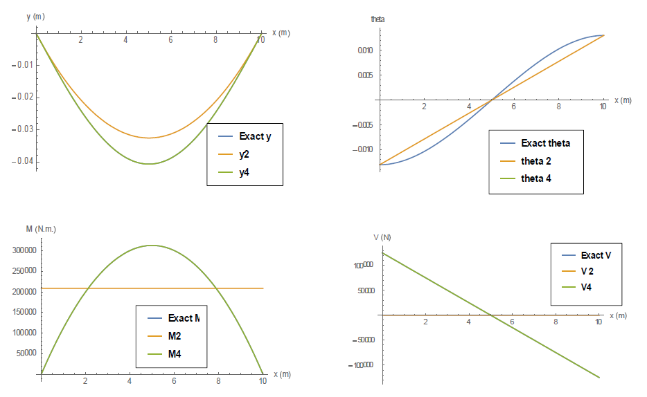
Similar to the previous examples, the coefficients are obtained by first satisfying the essential boundary conditions. Then, the remaining coefficients are obtained by minimizing the potential energy of the system. As shown in the plots below, the second and third degree trial functions give the same result, while the fourth and fifth degree trial functions give the same result. The solution is shown to give the accurate result when a polynomial of the fourth or higher degree is used.
(*Exact Solution*)
Clear[q,EI,y,x,c1,c2,c3,c4,L]
y=(q*x^4/24+c1*x^3/6+c2*x^2/2+c3*x+c4)/EI;
Eq1=y/.x-> 0;
Eq2=y/.x-> L;
Eq3=EI*D[y,{x,2}]/.x-> 0;
Eq4=EI*D[y,{x,2}]/.x-> L;
a=Solve[{Eq1==0,Eq2==0,Eq3==0,Eq4==0},{c1,c2,c3,c4}];
y=y/.a[[1]];
theta=D[y,x]/.a[[1]];
M=FullSimplify[EI*D[y,{x,2}]/.a[[1]]];
V=FullSimplify[EI*D[y,{x,3}]/.a[[1]]];
(*Second Degree*)
y2=a2*x^2+a1*x+a0;
s=Solve[{(y2/.x-> 0)==0,(y2/.x->L)==0},{a0,a1}];
y2=y2/.s[[1]];
theta2=D[y2,x];
M2=EI*D[y2,{x,2}];
V2=EI*D[y2,{x,3}];
PE=EI/2*Integrate[(D[y2,{x,2}])^2,{x,0,L}]-Integrate[q*y2,{x,0,L}];
Eq1=D[PE,a2];
a=Solve[{Eq1==0},{a2}];
y2=y2/.a[[1]];
theta2=D[y2,x]/.a[[1]];
M2=FullSimplify[EI*D[y2,{x,2}]/.a[[1]]];
V2=FullSimplify[EI*D[y2,{x,3}]/.a[[1]]];
(*Third Degree*)
y3=a3*x^3+a2*x^2+a1*x+a0;
s=Solve[{(y3/.x-> 0)==0,(y3/.x->L)==0},{a0,a1}];
y3=y3/.s[[1]];
theta3=D[y3,x];
M3=EI*D[y3,{x,2}];
V3=EI*D[y3,{x,3}];
PE=EI/2*Integrate[(D[y3,{x,2}])^2,{x,0,L}]-Integrate[q*y3,{x,0,L}];
Eq1=D[PE,a2];
Eq2=D[PE,a3];
a=Solve[{Eq1==0,Eq2==0},{a2,a3}];
y3=y3/.a[[1]];
theta3=D[y3,x]/.a[[1]];
M3=FullSimplify[EI*D[y3,{x,2}]/.a[[1]]];
V3=FullSimplify[EI*D[y3,{x,3}]/.a[[1]]];
(*fourth Degree*)
y4=a4*x^4+a3*x^3+a2*x^2+a1*x+a0;
s=Solve[{(y4/.x-> 0)==0,(y4/.x->L)==0},{a0,a1}];
y4=y4/.s[[1]];
theta4=D[y4,x];
M4=EI*D[y4,{x,2}];
V4=EI*D[y4,{x,3}];
PE=EI/2*Integrate[(D[y4,{x,2}])^2,{x,0,L}]-Integrate[q*y4,{x,0,L}];
Eq1=D[PE,a2];
Eq2=D[PE,a3];
Eq3=D[PE,a4];
a=Solve[{Eq1==0,Eq2==0,Eq3==0},{a2,a3,a4}];
y4=y4/.a[[1]];
theta4=D[y4,x]/.a[[1]];
M4=FullSimplify[EI*D[y4,{x,2}]/.a[[1]]];
V4=FullSimplify[EI*D[y4,{x,3}]/.a[[1]]];
(*fifth Degree*)
y5=a5*x^5+a4*x^4+a3*x^3+a2*x^2+a1*x+a0;
s=Solve[{(y5/.x-> 0)==0,(y5/.x->L)==0},{a0,a1}];
y5=y5/.s[[1]];
theta4=D[y5,x];
M5=EI*D[y5,{x,2}];
V5=EI*D[y5,{x,3}];
PE=EI/2*Integrate[(D[y5,{x,2}])^2,{x,0,L}]-Integrate[q*y5,{x,0,L}];
Eq1=D[PE,a2];
Eq2=D[PE,a3];
Eq3=D[PE,a4];
Eq4=D[PE,a5];
a=Solve[{Eq1==0,Eq2==0,Eq3==0,Eq4==0},{a2,a3,a4,a5}];
y5=y5/.a[[1]];
theta5=D[y5,x]/.a[[1]];
M5=FullSimplify[EI*D[y5,{x,2}]/.a[[1]]];
V5=FullSimplify[EI*D[y5,{x,3}]/.a[[1]]];
EI = 200000*1000000*4*100000000/1000000000000;
q = -25*1000;
L = 10;
Plot[{y,y2,y4},{x,0,L},AxesLabel-> {"x (m)","y (m)"},PlotLegends->{Style["Exact y",Bold,12],Style["y2",Bold,12],Style["y4",Bold,12]}]
Plot[{theta,theta2,theta4},{x,0,L},AxesLabel-> {"x (m)","theta"},PlotLegends-> {Style["Exact theta",Bold,12],Style["theta 2",Bold,12],Style["theta 4",Bold,12]}]
Plot[{M,M2,M4},{x,0,L},AxesLabel-> {"x (m)","M (N.m.)"},PlotLegends-> {Style["Exact M",Bold,12],Style["M2",Bold,12],Style["M4",Bold,12]}]
Plot[{V,V2,V4},{x,0,L},AxesLabel-> {"x (m)","V (N)"},PlotLegends->{Style["Exact V",Bold,12],Style["V 2",Bold,12],Style["V4",Bold,12]}]
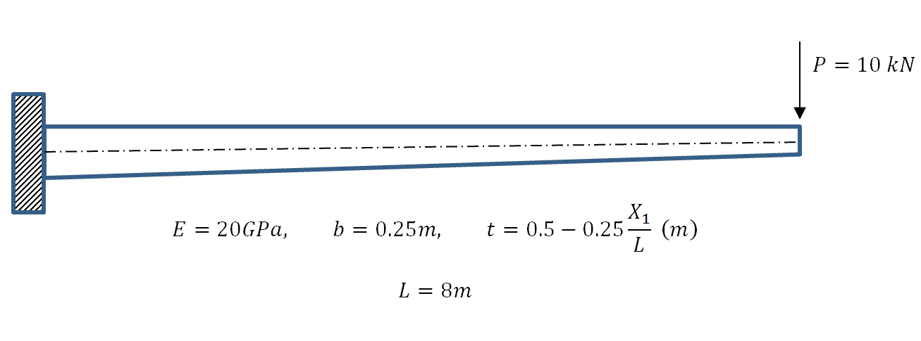
Example 3: Cantilever Beam with a Varying Cross Sectional Area
Let a beam with a length  and with a constant width
  and a linearly varying height (
 and
and  ) be aligned with the coordinate axis . Assume that the beam has a fixed left end and had a shearing load acting downwards of 10kN on its right end. Find the displacement, bending moment, and shearing force on the beam by directly solving the differential equation of equilibrium and then using the Rayleigh Ritz method assuming polynomials of the degrees (0, 1, 2, 3, 4, 5, 6, 7). Assume the beam to be linear elastic with Young’s modulus
  and that the Euler Bernoulli Beam is an appropriate beam approximation. Compare the Rayleigh Ritz method with the exact solution.
Solution
Exact Solution:
First, the exact solution that would satisfy the equilibrium equations can be obtained. The equilibrium equation as shown in the Euler Bernoulli beam section apply only when and are constant. Since is variable, the differential equation has the form:
![\[ \frac{\mathrm{d}^2\left(EI\frac{\mathrm{d}^2y}{\mathrm{d}X_1^2}\right)}{\mathrm{d}X_1^2}=q \]](https://engcourses-uofa.ca/wp-content/ql-cache/quicklatex.com-a431744379cace3cfa16e96db77aa508_l3.png "Rendered by QuickLaTeX.com")
For the cantilever beam, . For consistency in the units, in all the following calculations  and
and  N. The moment of inertia is a function of as follows:
![\[ I=\frac{bt^3}{12}=\frac{0.25\left(0.5-0.25\frac{X_1}{8}\right)^3}{12}=\frac{(16-X_1)^3}{1572864} \]](https://engcourses-uofa.ca/wp-content/ql-cache/quicklatex.com-96ee7b561ad24a508bd28c538acea832_l3.png "Rendered by QuickLaTeX.com")
The exact solution can be obtained using Mathematica. The following are the four boundary conditions required:
![\[ \begin{split} & @X_1=0:y=0\\ & @X_1=0:\theta=\frac{\mathrm{d}y}{\mathrm{d}X_1}=0\\ & @X_1=L:V=\frac{\mathrm{d}M}{\mathrm{d}X_1}=\frac{\mathrm{d}\left(EI\frac{\mathrm{d}^2y}{\mathrm{d}X_1^2}\right)}{\mathrm{d}X_1}=10000\\ & @X_1=L:M=EI\frac{\mathrm{d}^2y}{\mathrm{d}X_1^2}=0\\ \end{split} \]](https://engcourses-uofa.ca/wp-content/ql-cache/quicklatex.com-a02b5462dba19f6804183e87fd5d98f9_l3.png "Rendered by QuickLaTeX.com")
Using Mathematica, the above differential equation can be solved to yield the following exact solution for :
![\[ y=\frac{34.8872+(0.036864X_1-2.96688)X_1+(0.786432X_1-12.5829)\ln[16-X_1]}{X_1-16} \]](https://engcourses-uofa.ca/wp-content/ql-cache/quicklatex.com-710c2add20d685a2fd317375c0ce3dc0_l3.png "Rendered by QuickLaTeX.com")
The associated moment in N.m. and shearing force in N. are given by:
![\[ M=-80000+10000X_1\qquad V=10000 \]](https://engcourses-uofa.ca/wp-content/ql-cache/quicklatex.com-7f54e55ab8177a8e8a9f11171a0c9518_l3.png "Rendered by QuickLaTeX.com")
Obviously, as the beam is statically determinate, the equations for the moment and shear are very simple. However, the variable cross section leads to a complicated form for the displacement . Note that traditionally, in structural engineering applications, a constant cross section with the intermediate height of two thirds of the maximum height can be assumed to simplify the equations.
The Rayleigh Ritz Method:
The first step in the Rayleigh Ritz method finds the minimizer of the potential energy of the system which can be written as:
Notice that the potential energy lost by the action of the end force is equal to the product of ( is acting downwards and is assumed upwards) and the displacement evaluated at . To find an approximate solution, an assumption for the shape or the form of has to be introduced.
Polynomials of the Zero and First Degrees:
If we assume that is a constant (polynomial of the zero degree) or a linear (polynomial of the first degree) function, and when attempting to satisfy the essential boundary conditions:
this leads to the trivial solution , which will automatically be rejected.
Polynomial of the Second Degree:
The approximate solution forms for the displacement , the rotation , the moment , and the shear force functions if is assumed to be a polynomial of the second degree are:
![\[ \begin{split} y & =a_2X_1^2+a_1X_1+a_0\\ \theta &=\frac{\mathrm{d}y}{\mathrm{d}X_1} =2a_2X_1+a_1\\ M &=EI\frac{\mathrm{d}^2y}{\mathrm{d}X_1^2} =2EIa_2=-\frac{9765625}{384}a_2(-16+X_1)^3\\ V &=\frac{\mathrm{d}M}{\mathrm{d}X_1}=-\frac{9765625}{128}a_2(-16+X_1)^2 \end{split} \]](https://engcourses-uofa.ca/wp-content/ql-cache/quicklatex.com-cf9d505ba9685cd3a5d91499f507953e_l3.png "Rendered by QuickLaTeX.com")
To satisfy the essential boundary conditions, we have:
Therefore, the solutions forms have only one parameter that can be controlled:
![\[ \begin{split} y & =a_2X_1^2\\ \theta &=\frac{\mathrm{d}y}{\mathrm{d}X_1} =2a_2X_1\\ M &=EI\frac{\mathrm{d}^2y}{\mathrm{d}X_1^2} =2EIa_2=-\frac{9765625}{384}a_2(-16+X_1)^3\\ V &=\frac{\mathrm{d}M}{\mathrm{d}X_1}=-\frac{9765625}{128}a_2(-16+X_1)^2 \end{split} \]](https://engcourses-uofa.ca/wp-content/ql-cache/quicklatex.com-84a024cb32dc11b93bab2a954c31982d_l3.png "Rendered by QuickLaTeX.com")
Substituting into the equation of the potential energy of an Euler Bernoulli beam:
![\[\begin{split} PE&=\int_0^L\!\frac{EI}{2} \left(2a_2\right)^2\,\mathrm{d}X_1+P\left(a_2L^2\right)=\int_0^L\!\frac{9765625a_2^2(16-X_1)^3}{384}\,\mathrm{d}X_1+640000a_2\\ &=640000a_2+390625000a_2^2 \end{split} \]](https://engcourses-uofa.ca/wp-content/ql-cache/quicklatex.com-8e89639486d0fbc7eebe84989089d764_l3.png "Rendered by QuickLaTeX.com")
Note that is a function of and so it stays inside the integral. The unknown coefficient can be obtained by minimizing the potential energy:
![\[ \frac{\mathrm{d} PE}{\mathrm{d} a_2} =0\Rightarrow a_2=\frac{-64}{78125} \]](https://engcourses-uofa.ca/wp-content/ql-cache/quicklatex.com-7b2604f794dff19ad534aba3fe16ecaf_l3.png "Rendered by QuickLaTeX.com")
Therefore, the “best” parabolic approximation for along with the corresponding solutions for and are given by:
![\[ \begin{split} y & =\frac{-64}{78125}X_1^2=-0.0008192X_1^2\\ M &=EI\frac{\mathrm{d}^2y}{\mathrm{d}X_1^2} =\frac{125}{6}(X_1-16)^3\\ &=-85333.3 + 16000 X_1 - 1000 X_1^2 + 20.8333 X_1^3\\ V &=\frac{\mathrm{d}M}{\mathrm{d}X_1} =\frac{125}{2}(X_1-16)^2\\ &=16000 - 2000 X_1 + 62.5 X_1^2 \end{split} \]](https://engcourses-uofa.ca/wp-content/ql-cache/quicklatex.com-7d221e63e9ab4df9e3f4bdca076a8322_l3.png "Rendered by QuickLaTeX.com")
Polynomial of the Third Degree:
The approximate solution forms for the displacement , the rotation , the moment , and the shear force functions if is assumed to be a polynomial of the third degree are:
![\[ \begin{split} y & =a_3X_1^3+a_2X_1^2+a_1X_1+a_0\\ \theta &=\frac{\mathrm{d}y}{\mathrm{d}X_1} =3a_3X_1^2+2a_2X_1+a_1\\ M &=EI\frac{\mathrm{d}^2y}{\mathrm{d}X_1^2} =6EIa_3X_1+2EIa_2\\ V &=\frac{\mathrm{d}M}{\mathrm{d}X_1} \end{split} \]](https://engcourses-uofa.ca/wp-content/ql-cache/quicklatex.com-cfd5bdb5921ecf684a7b628846648c45_l3.png "Rendered by QuickLaTeX.com")
To satisfy the essential boundary conditions, we have:
Therefore, the solutions forms have only two parameters and that can be controlled:
![\[ \begin{split} y & =a_3X_1^3+a_2X_1^2\\ \theta &=\frac{\mathrm{d}y}{\mathrm{d}X_1} =3a_3X_1^2+2a_2X_1\\ M &=EI\frac{\mathrm{d}^2y}{\mathrm{d}X_1^2} =6EIa_3X_1+2EIa_2=-\frac{9765625}{384}(-16+X_1)^3(a_2+3a_3X_1)\\ V &=-\frac{9765625}{128}(-16+X_1)^2(a_2+4a_3(X_1-4)) \end{split} \]](https://engcourses-uofa.ca/wp-content/ql-cache/quicklatex.com-1e5e1a091aada49ef325682b004c78c6_l3.png "Rendered by QuickLaTeX.com")
Substituting into the equation of the potential energy of an Euler Bernoulli beam:
![\[ PE=\int_0^L\!\frac{EI}{2}\left(6a_3X_1+2a_2\right)^2\,\mathrm{d}X_1+P\left(a_3L^3+a_2L^2\right) \]](https://engcourses-uofa.ca/wp-content/ql-cache/quicklatex.com-90e291c95e3b2e2f1f8e3335df1d47fb_l3.png "Rendered by QuickLaTeX.com")
The unknown coefficients and can be obtained by minimizing the potential energy:
![\[\begin{split} \frac{\partial PE}{\partial a_2} & =640000+781250000a_2+6500000000a_3=0\\ \frac{\partial PE}{\partial a_3} & =5120000+6500000000a_2+84000000000a_3=0 \end{split} \]](https://engcourses-uofa.ca/wp-content/ql-cache/quicklatex.com-09d4e7b1dca10d8364cf7fbf93718080_l3.png "Rendered by QuickLaTeX.com")
Solving the above two equations yields:
![\[ a_2=-\frac{512}{584375} \qquad a_3=\frac{4}{584375} \]](https://engcourses-uofa.ca/wp-content/ql-cache/quicklatex.com-3ba5ac04545ebfd8fb28ce7cdeb5dc12_l3.png "Rendered by QuickLaTeX.com")
Therefore, the “best” cubic approximation for along with the corresponding solutions for , , and are given by:
![\[ \begin{split} y & =\frac{4X_1^3}{584375}-\frac{512X_1^2}{584375}\\ &=-0.00087615X_1^2+6.84492(10)^{-6}X_1^3\\ M &=EI\frac{\mathrm{d}^2y}{\mathrm{d}X_1^2} =-\frac{3125(-16+X_1)^3(-128+3X_1)}{17952}\\ &=-91265.6 + 19251.3 X_1 - 1470.59 X_1^2 + 47.3485 X_1^3 - 0.522226 X_1^4\\ V &=\frac{\mathrm{d}M}{\mathrm{d}X_1} =-\frac{3125(-36+X_1)(-16+X_1)^2}{1496}\\ &=19251.3 - 2941.18 X_1 + 142.045 X_1^2 - 2.0889 X_1^3 \end{split} \]](https://engcourses-uofa.ca/wp-content/ql-cache/quicklatex.com-4d7758cda3398590a54cfcb801fbe544_l3.png "Rendered by QuickLaTeX.com")
Polynomials of the Fourth Degree:
The approximate solution forms for the displacement , the rotation , the moment , and the shear force functions if is assumed to be a polynomial of the fourth degree are:
![\[ \begin{split} y & =a_4X_1^4+a_3X_1^3+a_2X_1^2+a_1X_1+a_0\\ \theta &=\frac{\mathrm{d}y}{\mathrm{d}X_1} =4a_4X_1^3+3a_3X_1^2+2a_2X_1+a_1\\ M &=EI\frac{\mathrm{d}^2y}{\mathrm{d}X_1^2} =12EIa_4X_1^2+6EIa_3X_1+2EIa_2\\ V &=\frac{\mathrm{d}M}{\mathrm{d}X_1} \end{split} \]](https://engcourses-uofa.ca/wp-content/ql-cache/quicklatex.com-8153447efff6148225db22985f3fa3ae_l3.png "Rendered by QuickLaTeX.com")
To satisfy the essential boundary conditions, we have:
Therefore, the solutions forms have the parameters , , and that can be controlled:
![\[ \begin{split} y & =a_4X_1^4+a_3X_1^3+a_2X_1^2\\ M &=EI\frac{\mathrm{d}^2y}{\mathrm{d}X_1^2} =12EIa_4X_1^2+6EIa_3X_1+2EIa_2\\ V &=\frac{\mathrm{d}M}{\mathrm{d}X_1} \end{split} \]](https://engcourses-uofa.ca/wp-content/ql-cache/quicklatex.com-599d43bb0ece5dede714e77d9f13b6ef_l3.png "Rendered by QuickLaTeX.com")
Substituting into the equation of the potential energy of an Euler Bernoulli beam:
![\[ PE=\int_0^L\!\frac{EI}{2}\left(12a_4X_1^2+6a_3X_1+2a_2\right)^2\,\mathrm{d}X_1+P\left(a_4L^4+a_3L^3+a_2L^2\right) \]](https://engcourses-uofa.ca/wp-content/ql-cache/quicklatex.com-ce52ae904258afe8738992db9c814bba_l3.png "Rendered by QuickLaTeX.com")
The unknown coefficients , , and can be obtained by minimizing the potential energy:
Solving the above three equations yields:
![\[ a_2=-0.000704051 \qquad a_3=-0.0000484584 \qquad a_4=-4.01821(10)^{-6} \]](https://engcourses-uofa.ca/wp-content/ql-cache/quicklatex.com-6672c4906236904a614157a8491c8b47_l3.png "Rendered by QuickLaTeX.com")
Therefore, assuming a fourth order polynomial gives the following set of solutions:
![\[ \begin{split} y & =-0.000704051X_1^2-0.0000484584X_1^3+4.01821(10)^{-6}X_1^4\\ M &=EI\frac{\mathrm{d}^2y}{\mathrm{d}X_1^2} =-73338.7 - 1392.24 X_1 + 4491.3 X_1^2 - 630.438 X_1^3 + 33.1273 X_1^4 - 0.61313 X_1^5\\ V &=\frac{\mathrm{d}M}{\mathrm{d}X_1}=-1392.24 + 8982.6 X_1 - 1891.32 X_1^2 + 132.509 X_1^3 - 3.06565 X_1^4 \end{split} \]](https://engcourses-uofa.ca/wp-content/ql-cache/quicklatex.com-bf9447d5935393a17cf1ca26789e3afa_l3.png "Rendered by QuickLaTeX.com")
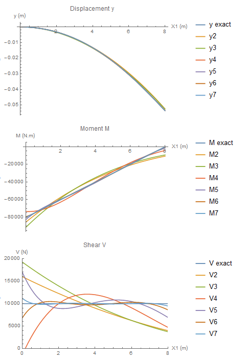
Approximate solutions using higher order polynomials can be obtained similarly. The following plots show the convergence of the polynomial functions to the exact solution up to a polynomial of the sixth degree (Mathematica code is given below). In the first plot, it is clear that a polynomial of the second degree is capable of capturing the displacement quite accurately. However, the corresponding approximate solutions for the moment and shear are not as accurate. The accuracy of the approximate solution for the bending moment is higher than that for the shearing force and that is because the moment is related to the second derivative of while the shear is related to the third derivative of . It takes up to a polynomial of the seventh degree for for the approximate shearing force to have a flat distribution similar to the exact solution.
View Mathematica Code
Clear[y, b, L, t, Ii, Ee, P]
b = 1/4;
L = 8;
t = (1/2 - 1/4*X1/L);
Ii = b*t^3/12;
Ee = 20*10^9;
P = 10000;
a = DSolve[{D[Ee*Ii*y''[X1], {X1, 2}] == 0, y[0] == 0, y'[0] == 0, y''[L] == 0, (D[Ee*Ii, X1] /. X1 -> L)*y''[L] + (Ee*Ii /. X1 -> L)*y'''[L] == P}, y[X1], X1, Assumptions -> 0 <= X1 <= L]
y = FullSimplify[Chop[N[y[X1] /. a[[1]]]]]
th = D[y, X1];
M = FullSimplify[Ee*Ii*D[y, {X1, 2}]]
V = FullSimplify[D[M, X1]]

Plot[y, {X1, 0, L}, PlotLabel -> "Displacement y", AxesLabel -> {"X1 (m)", "y (m)"}, PlotLegends -> {"y exact"}]
Plot[M, {X1, 0, L}, PlotLabel -> "Moment M", AxesLabel -> {"X1 (m)", "M (N.m)"}, PlotLegends -> {"M exact"}]
Plot[V, {X1, 0, L}, PlotRange -> {{0, L}, {0, 2 P}}, PlotLabel -> "Shear V", AxesLabel -> {"X1 (m)", "V (N)"}, PlotLegends -> {"V exact"}]

Print["Second Order Polynomial"]
y2 = a2*X1^2;
d2y = D[y2, {X1, 2}];
PE = Integrate[Ee*Ii/2*d2y^2, {X1, 0, L}] - (-P)*y2 /. X1 -> L;
sol = Solve[D[PE, a2] == 0, a2]
y2 = y2 /. sol[[1]]
M2 = FullSimplify[Ee*Ii*D[y2, {X1, 2}]]
V2 = FullSimplify[D[M2, X1]]
Plot[{y, y2}, {X1, 0, L}, PlotLabel -> "Displacement y", AxesLabel -> {"X1 (m)", "y (m)"}, PlotLegends -> {"y exact", "y2"}]
Plot[{M, M2}, {X1, 0, L}, PlotLabel -> "Moment M", AxesLabel -> {"X1 (m)", "M (N.m)"}, PlotLegends -> {"M exact", "M2"}]
Plot[{V, V2}, {X1, 0, L}, PlotRange -> {{0, L}, {0, 2 P}}, PlotLabel -> "Shear V", AxesLabel -> {"X1 (m)", "V (N)"}, PlotLegends -> {"V exact", "V2"}]

Print["Third Order Polynomial"]
y3 = a2*X1^2 + a3*X1^3;
d2y = D[y3, {X1, 2}];
PE = Integrate[Ee*Ii/2*d2y^2, {X1, 0, L}] - (-P)*y3 /. X1 -> L;
sol = Solve[{D[PE, a2] == 0, D[PE, a3] == 0}, {a2, a3}]
y3 = y3 /. sol[[1]]
M3 = FullSimplify[Ee*Ii*D[y3, {X1, 2}]]
V3 = FullSimplify[D[M3, X1]]
Plot[{y, y3}, {X1, 0, L}, PlotLabel -> "Displacement y", AxesLabel -> {"X1 (m)", "y (m)"}, PlotLegends -> {"y exact", "y3"}]
Plot[{M, M3}, {X1, 0, L}, PlotLabel -> "Moment M", AxesLabel -> {"X1 (m)", "M (N.m)"}, PlotLegends -> {"M exact", "M3"}]
Plot[{V, V3}, {X1, 0, L}, PlotRange -> {{0, L}, {0, 2 P}}, PlotLabel -> "Shear V", AxesLabel -> {"X1 (m)", "V (N)"},  PlotLegends -> {"V exact", "V3"}]

Print["Fourth Order Polynomial"]
y4 = a2*X1^2 + a3*X1^3 + a4*X1^4;
d2y = D[y4, {X1, 2}];
PE = Integrate[Ee*Ii/2*d2y^2, {X1, 0, L}] - (-P)*y4 /. X1 -> L;
sol = Solve[{D[PE, a2] == 0, D[PE, a3] == 0, D[PE, a4] == 0}, {a2, a3, a4}]
y4 = y4 /. sol[[1]]
M4 = FullSimplify[Ee*Ii*D[y4, {X1, 2}]]
V4 = FullSimplify[D[M4, X1]]
Plot[{y, y4}, {X1, 0, L}, PlotLabel -> "Displacement y", AxesLabel -> {"X1 (m)", "y (m)"}, PlotLegends -> {"y exact", "y4"}]
Plot[{M, M4}, {X1, 0, L}, PlotLabel -> "Moment M", AxesLabel -> {"X1 (m)", "M (N.m)"}, PlotLegends -> {"M exact", "M4"}]
Plot[{V, V4}, {X1, 0, L}, PlotRange -> {{0, L}, {0, 2 P}}, PlotLabel -> "Shear V", AxesLabel -> {"X1 (m)", "V (N)"}, PlotLegends -> {"V exact", "V4"}]

Print["Fifth Order Polynomial"]
y5 = a2*X1^2 + a3*X1^3 + a4*X1^4 + a5*X1^5;
d2y = D[y5, {X1, 2}];
PE = Integrate[Ee*Ii/2*d2y^2, {X1, 0, L}] - (-P)*y5 /. X1 -> L;
sol = Solve[{D[PE, a2] == 0, D[PE, a3] == 0, D[PE, a4] == 0, D[PE, a5] == 0}, {a2, a3, a4, a5}]
y5 = y5 /. sol[[1]]
M5 = FullSimplify[Ee*Ii*D[y5, {X1, 2}]]
V5 = FullSimplify[D[M5, X1]]
Plot[{y, y5}, {X1, 0, L}, PlotLabel -> "Displacement y", AxesLabel -> {"X1 (m)", "y (m)"}, PlotLegends -> {"y exact", "y5"}]
Plot[{M, M5}, {X1, 0, L}, PlotLabel -> "Moment M",  AxesLabel -> {"X1 (m)", "M (N.m)"}, PlotLegends -> {"M exact", "M5"}]
Plot[{V, V5}, {X1, 0, L}, PlotRange -> {{0, L}, {0, 2 P}}, PlotLabel -> "Shear V", AxesLabel -> {"X1 (m)", "V (N)"}, PlotLegends -> {"V exact", "V5"}]

Print["Sixth Order Polynomial"]
y6 = a2*X1^2 + a3*X1^3 + a4*X1^4 + a5*X1^5 + a6*X1^6;
d2y = D[y6, {X1, 2}];
PE = Integrate[Ee*Ii/2*d2y^2, {X1, 0, L}] - (-P)*y6 /. X1 -> L;
sol = Solve[{D[PE, a2] == 0, D[PE, a3] == 0, D[PE, a4] == 0, D[PE, a5] == 0, D[PE, a6] == 0}, {a2, a3, a4, a5, a6}]
y6 = y6 /. sol[[1]]
M6 = FullSimplify[Ee*Ii*D[y6, {X1, 2}]]
V6 = FullSimplify[D[M6, X1]]
Plot[{y, y6}, {X1, 0, L}, PlotLabel -> "Displacement y",  AxesLabel -> {"X1 (m)", "y (m)"}, PlotLegends -> {"y exact", "y6"}]
Plot[{M, M6}, {X1, 0, L}, PlotLabel -> "Moment M",  AxesLabel -> {"X1 (m)", "M (N.m)"}, PlotLegends -> {"M exact", "M6"}]
Plot[{V, V6}, {X1, 0, L}, PlotRange -> {{0, L}, {0, 2 P}},  PlotLabel -> "Shear V", AxesLabel -> {"X1 (m)", "V (N)"},  PlotLegends -> {"V exact", "V6"}]

Print["Seventh Order Polynomial"]
y7 = a2*X1^2 + a3*X1^3 + a4*X1^4 + a5*X1^5 + a6*X1^6 + a7*X1^7;
d2y = D[y7, {X1, 2}];
PE = Integrate[Ee*Ii/2*d2y^2, {X1, 0, L}] - (-P)*y7 /. X1 -> L;
sol = Solve[{D[PE, a2] == 0, D[PE, a3] == 0, D[PE, a4] == 0, D[PE, a5] == 0, D[PE, a6] == 0, D[PE, a7] == 0}, {a2, a3, a4, a5,a6, a7}]
y7 = y7 /. sol[[1]]
M7 = FullSimplify[Ee*Ii*D[y7, {X1, 2}]]
V7 = FullSimplify[D[M7, X1]]
Plot[{y, y7}, {X1, 0, L}, PlotLabel -> "Displacement y", AxesLabel -> {"X1 (m)", "y (m)"}, PlotLegends -> {"y exact", "y7"}]
Plot[{M, M7}, {X1, 0, L}, PlotLabel -> "Moment M",  AxesLabel -> {"X1 (m)", "M (N.m)"}, PlotLegends -> {"M exact", "M7"}]
Plot[{V, V7}, {X1, 0, L}, PlotRange -> {{0, L}, {0, 2 P}},  PlotLabel -> "Shear V", AxesLabel -> {"X1 (m)", "V (N)"}, PlotLegends -> {"V exact", "V7"}]


Plot[{y, y2, y3, y4, y5, y6, y7}, {X1, 0, L},  PlotLabel -> "Displacement y", AxesLabel -> {"X1 (m)", "y (m)"},  PlotLegends -> {"y exact", "y2", "y3", "y4", "y5", "y6", "y7"}]
Plot[{M, M2, M3, M4, M5, M6, M7}, {X1, 0, L}, PlotLabel -> "Moment M",  AxesLabel -> {"X1 (m)", "M (N.m)"},  PlotLegends -> {"M exact", "M2", "M3", "M4", "M5", "M6", "M7"}]
Plot[{V,V2,V3,V4,V5,V6,V7}, {X1, 0, L}, PlotRange ->{{0, L}, {0, 2 P}},PlotLabel->"Shear V",AxesLabel -> {"X1 (m)", "V (N)"},PlotLegends -> {"V exact", "V2", "V3", "V4", "V5", "V6", "V7"}]
Problems
- The exact displacement in meters of the shown Euler Bernoulli beam follows the function:
![\[ y=\begin{cases} 0.0003375X_1^2(3X_1-20) & 0\leq X_1\leq 5\\ -0.0003125(X_1-8)^2(7X_1-20) & 5< X_1\leq 8 \end{cases} \]](https://engcourses-uofa.ca/wp-content/ql-cache/quicklatex.com-3c6a4edaf6b4d8ac5fe52b9cb8ed4e2a_l3.png "Rendered by QuickLaTeX.com")
The beam’s Young’s modulus and moment of inertia are
 and
and  .
.
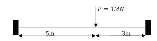
- Find the strain energy stored in the beam (Answer: 21093.8 N.m.).
- Use the Rayleigh Ritz method to find approximate solutions for the displacement across the whole beam. Assume the approximations to be polynomials of the zero, first, second, third, fourth, fifth, and sixth degrees.
- Plot the exact solution versus the approximate solutions for , , , and . Comment on the results.
- For the following two linear elastic isotropic small deformations beam structures:
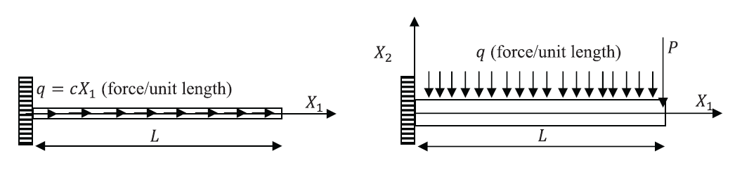
- Find the exact solution of the displacement.
- Find an approximate solution using the Rayleigh Ritz method with polynomial trial functions of zero, first, second, third, and fourth degrees satisfying the essential boundary conditions. Comment on the difference between the approximate and the exact solutions.
- An Euler Bernoulli beam of length with both ends fixed is loaded by a concentrated force at the centre of the beam. Assume that the beam is made out of a linear elastic isotropic material and that the deformations are small. If is Young’s modulus and is the moment of inertia, then find:
- the strain energy in terms of the displacement function .
- The expression for the potential energy of the system.
- Show that the following series satisfies the essential boundary conditions
![\[ w=\sum_{n=2}^\infty A_n\left(\cos{\frac{n\pi x}{L}}-1\right) \]](https://engcourses-uofa.ca/wp-content/ql-cache/quicklatex.com-86ccd54894e41abfabfe533b8d3a5be7_l3.png "Rendered by QuickLaTeX.com")
where
 and
and  are constants
 - Take one term and two terms from the series above and determine the constants using the Rayleigh Ritz method.
- Find the exact solution and compare with the approximate solutions obtained using the Rayleigh Ritz method.
- the strain energy in terms of the displacement function
- For the shown two beam structures
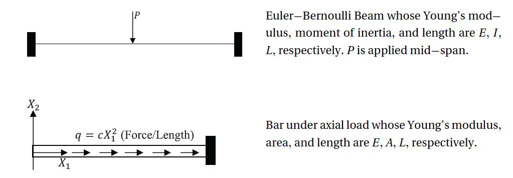
- Find the exact solution for the displacement.
- Use the Rayleigh Ritz method with polynomials of the zero, one, two, three, four, five, and six degrees to find an approximate solution for the displacement. For the beam under axial loading compare the stresses with the exact solution. For the beam under lateral loading, compare the rotation, moment, and shear with the corresponding exact solutions.
- The shown beam under axial loading is subjected to the varying body force given per unit volume. Assume that the area varies linearly across the length of the structure.
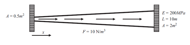
- Find the exact displacement by solving the differential equation of equilibrium for bars under axial loading.
- Use the Rayleigh Ritz method to find a polynomial approximation of the zero, first, second, and third degrees for the displacement function.
- The shown plate has a thickness
 . The plate is in a plane stress condition. The left boundary where has zero vertical and horizontal displacements. The material is linear elastic with small deformations and Young’s modulus and Poisson’s ratio
  are equal to 200 GPa and 0.3, respectively. The right boundary is subjected to a constant normal tensile stress of 20MPa while the bottom boundary is subjected to a normal compressive stress that varies linearly with a maximum value of 20MPa as shown in the figure below. Using the Rayleigh Ritz method and assuming that the displacement of the plate can be approximated using the function:
![\[ u=\left(\begin{array}{c}a_0+a_1X_1+a_2X_2+a_3X_1X_2\\b_0+b_1X_1+b_2X_2+b_3X_1X_2\end{array}\right) \]](https://engcourses-uofa.ca/wp-content/ql-cache/quicklatex.com-e6f95de756efd831cb7c5f2800b1d587_l3.png "Rendered by QuickLaTeX.com")
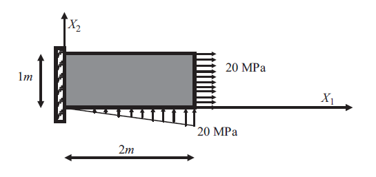
- Utilize the essential boundary conditions to reduce the number of unknown constants in the displacement function.
- Find the infinitesimal strain tensor in terms of the remaining unknown constants.
- Write the expression of the potential energy of the system in terms of the remaining unknown constants.
- Find the unknown constants using the Rayleigh Ritz method.
- Comment on how accurate the above displacement function is in approximating the exact displacement of the plate.
- Consider a uniaxial bar of length , Young’s modulus , and variable cross sectional area
 . The bar is fixed at one end and free at the other end. The free end is subjected to a constant force
  . Using the Rayleigh Ritz method, and assuming a trial parabolic displacement function
  , determine the approximate displacement function of the bar. Compare the results with the exact solution given by:
![\[ u=\frac{FL}{EA_0}\ln\left(1+\frac{x}{L}\right) \]](https://engcourses-uofa.ca/wp-content/ql-cache/quicklatex.com-cc2ba9a7ca04dc3b3f14571cad1a17ab_l3.png "Rendered by QuickLaTeX.com")
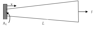
- Two bars joined at
 are subjected to a force at the joint. The cross sectional area of the larger bar is twice that of the smaller bar. Use the Rayleigh Ritz method with a trial displacement function of to approximate the exact displacement of the bar. Assume the area of the smaller bar to be equal to 10
 ,
,  ,
,  , and
, and  . Compare with the exact displacement field.
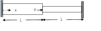
- A beam of length Young’s modulus , and moment of inertia is fixed at both ends and subjected to a uniformly distributed load and a concentrated force at midspan. Use the Rayligh Ritz method with a trial function
 where is a real number to approximate the midspan deflection of the beam.
 - Consider a uniaxial bar of length , Young’s modulus , and variable cross sectional area
 . The bar is fixed at one end and free at the other end. The free end is subjected to a constant force and a uniformly distributed force . Using the Rayleigh Ritz method, and assuming a quadratic trial displacement function, determine the approximate displacement of the bar.