Engineering at Alberta Courses » Single Degree of Freedom

Energy: Single Degree of Freedom

In this section we will investigate the static and dynamic equilibria of a single degree of freedom mass-spring system. Under static static equilibrium of such system, loading of the system gives rise to an energy of deformation (termed potential energy) that is stored in the spring. This energy is released upon removal of loading. In the case of dynamic equilibrium of such system, the energy of the system is composed of two terms whose sum is constant, the kinetic energy due to the velocity of the mass and the potential energy (energy of deformation) stored in the spring. The presentation of the single degree of freedom, while elementary, enables the extension of the same principles to the deformation of continuum objects.

Static Equilibrium of a Mass-Spring System:

The equilibrium of a mass-spring system is achieved when the weight of the mass is equal to the force applied in the spring. In other words equilibrium is achieved when:

$f(x)=mg$

where $x$ is the displacement (extension/contraction) of the spring, $f(x)$ is the force in the spring which is function of the displacement, $m$ is the mass of the spring, and $g$ is the gravity body force per unit mass (The ground acceleration). The displacement $x$ at which equilibrium is achieved is going to be termed $\Delta$ . In the following, we will investigate three forms for the force function $f(x)$ ; linear elastic, nonlinear elastic, and non-elastic.

Linear Elastic Spring:

A linear elastic spring has a linear relationship between the spring force $f$ and the displacement $x$ such that $f=kx$ where $k$ has units of force/unit length. When a weight of value $mg$ is gradually hung the spring is gradually stretched until equilibrium is achieved when $x=\Delta$ . At this stage, the spring force is equal to the applied weight and thus:

$k\Delta=mg$

The work done by the external forces during the process of loading is stored as an elastic potential energy inside the spring and can be recovered once the load is removed (Figure 1). The spring force acts to reduce the potential energy of the spring by always acting to reduce the spring length to its original unstretched length. At an arbitrary distance x, the potential energy stored in the spring is equal to

$\overline{U}=\int_0^x \! f(x) \, \mathrm{d}x = \int_0^x \! kx \, \mathrm{d}x = \frac{1}{2} k x^2$

In the process of moving a distance $x$ downward, the weight $mg$ lost some of its gravitational potential energy that is equal to the value $mgx$ . We call this term the work done by the external load. If we consider the combined system of the spring and the mass, then the potential energy of the system is equal to:

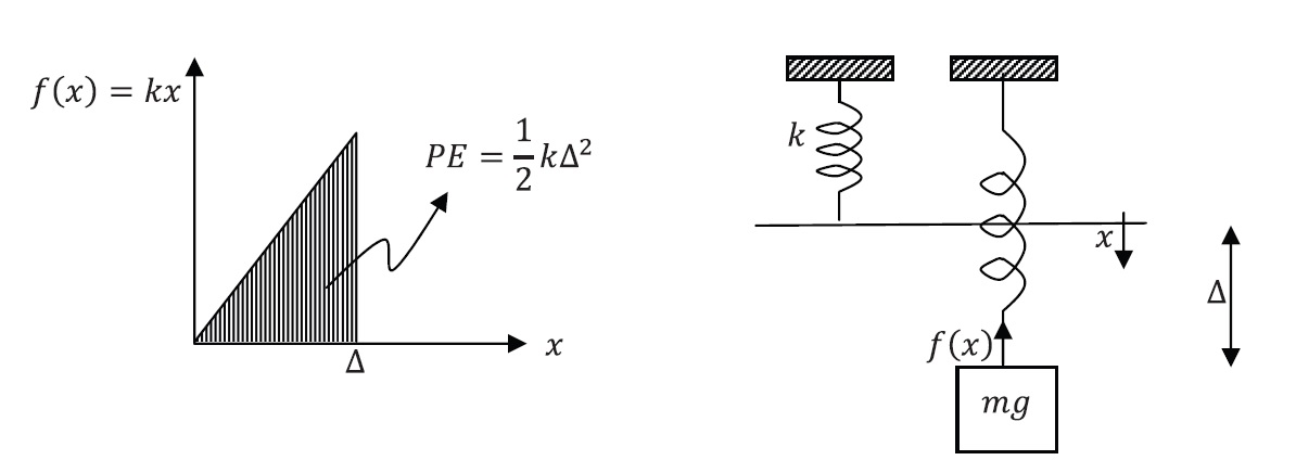
(1) $\begin{equation*} PE=\overline{U} - \mbox{Work Done by external load} = \frac{1}{2} kx^2-mgx \end{equation*}$

Figure 1. Mass – Linear Elastic Spring System

The potential energy of the system can be viewed also as the resulting expression when integrating the equilibrium equation from 0 to $x$ :

$f(x)-mg=0\Rightarrow PE=\int_0^x \! kx-mg \, \mathrm{d}x =\frac{1}{2} kx^2-mgx$

Therefore, differentiating the potential energy function leads to the equilibrium equation:

$\frac{\mathrm{d}PE}{\mathrm{d}x}=kx-mg$

The potential energy is a function of the displacement $x$ of the spring. When the displacement $x=\Delta$ , the rate of change of the potential energy is equal to zero:

$\frac{\mathrm{d}PE}{\mathrm{d}x}\bigg|_{x=\Delta}=k\Delta-mg=0$

Therefore, at equilibrium, the potential energy function is either a maximum, minimum, or an inflection point. To identify which of the three, we can take the second derivative of the potential energy:

$\frac{\mathrm{d}^2PE}{\mathrm{d}x^2}=k$

Therefore, the stiffness of the spring is what determines whether the potential energy is minimum, maximum, or an inflection point. When $k$ is positive, the potential energy of the system is minimum at equilibrium!

Nonlinear Elastic Spring:

A nonlinear elastic spring has a nonlinear relationship between the spring force $f(x)$ and the displacement $x$ . When a weight of value $mg$ is gradually hung the spring is gradually stretched until equilibrium is achieved when $x=\Delta$ . At this stage, the spring force is equal to the applied weight and thus:

$f(\Delta)=mg$

Similar to the linear case, the work done by the external forces during the process of loading is stored as an elastic potential energy inside the spring and can be recovered once the load is removed. The spring force acts to reduce the potential energy of the spring by always acting to reduce the spring length to its original unstretched length. At an arbitrary distance x, the potential energy stored in the spring is equal to

$\overline{U}=\int_0^x \! f(x) \, \mathrm{d}x$

Similar to the linear case, the potential energy of the system is equal to:

$PE=\overline{U} - \mbox{Work Done by external load} = \int_0^x \! f(x) \, \mathrm{d}x -mgx$

The potential energy of the system can be viewed also as the resulting expression when integrating the equilibrium equation from 0 to $x$ :

$f(x)-mg=0\Rightarrow PE=\int_0^x \! f(x)-mg \, \mathrm{d}x =\int_0^x \! f(x) \, \mathrm{d}x-mgx$

Therefore, differentiating the potential energy function leads to the equilibrium equation:

$\frac{\mathrm{d}PE}{\mathrm{d}x}=f(x)-mg$

The potential energy is a function of the displacement $x$ of the spring. When the displacement $x=\Delta$ , the rate of change of the potential energy is equal to zero:

$\frac{\mathrm{d}PE}{\mathrm{d}x}\bigg|_{x=\Delta}=f(\Delta)-mg=0$

$\frac{\mathrm{d}^2PE}{\mathrm{d}x^2}=f'(x)$

Therefore, the slope of the force displacement curve of the spring is what determines whether the potential energy is minimum, maximum, or an inflection point. When $f'$ is positive, the potential energy of the system is minimum at equilibrium while when $f'$ is negative, the potential energy is maximum! In addition, when the slope of the spring force is negative with respect to the displacement $x$ , the equilibrium position is deemed unstable. In this case, under the effect of an external force $F$ , any small perturbation in the displacement would lead to instabilities in the system. To understand this, let there be an equilibrium position $x_1$ where the slope is negative (Figure 2c & d). At this instance, the external force $F$ is in equilibrium with the internal spring force $f(x_1)$ . Imagine then, that a small perturbation in the displacement increases the position to $x_2$ corresponding to an internal force $f(x_2)$ . Since the slope is negative, $f(x_2)<f(x_1)=F$ . This, in turn, will lead to further extension in the direction of the higher force $F$ . Thus, the system will become unstable with the external force $F$ acting to increase the extension x in an unstable fashion.

Note that if the extension of the spring is applied using a displacement-controlling mechanism, this unstable mechanism will not be observed.

On the other hand, a spring whose force is always increasing with respect to the displacement (Figures 2a and 2b), and if the external load is not a function of the displacement $x$ then this spring is always stable and the mathematical expression for that is:

$\frac{\mathrm{d}^2PE}{\mathrm{d}x^2}=\frac{\mathrm{d}f(x)}{\mathrm{d}x}>0$

A continuously smooth function whose second derivative is always higher than zero belongs to the family of “convex” functions. If the elastic strain energy density of continuum bodies is convex in its variables, this implies that the material is stable.

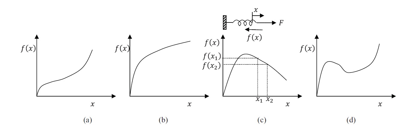
Figure 2. Force versus extension in nonlinear elastic springs. (a) and (b) Slope is always positive, and the potential energy is minimum at the equilibrium position. (c) and (d) have negative slopes in some portions, and thus, at those locations, any perturbation in the displacement would lead to instabilities and loss of equilibrium.

Non-Elastic Spring:

The term nonelastic spring implies that the force in the spring is not simply a function of the position only but of the history of loading as well. For example, during a cycle of loading, the energy supplied by external sources dissipates in the system or turns into a form that is not useful. Figure 3 shows an elasto-plastic spring during a cycle of gradual loading and unloading. When the mass is gradually removed, the spring does not return back to its original position, but has a residual extension $\Delta_{plastic}$ . The energy required to reach from state A to state B is the area under the curve shown in Figure 3b. During unloading, the load displacement curve follows a different path and some energy is lost. As can be seen in state C shown in Figure 3, the energy lost during the loading cycle is manifested in some change in the internal structure of the spring, which now has a longer length than that before loading. In such springs, a potential energy function cannot be easily defined, and the behaviour of the spring is history (path) dependent.

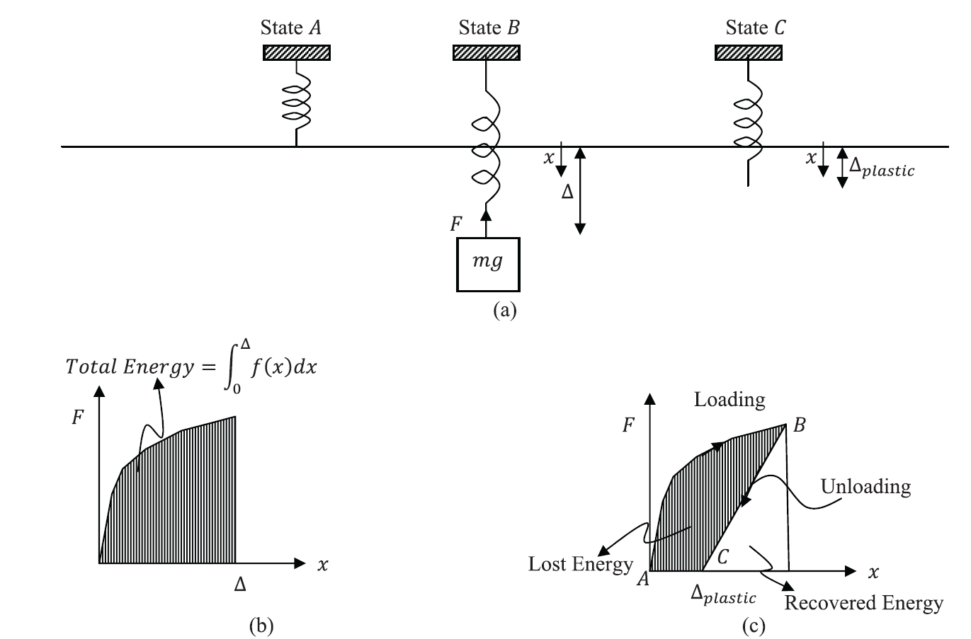
A cycle of loading and unloading in an elasto-plastic spring. (a) The process of loading and unloading produces a residual plastic extension, (b) energy supplied to the spring during the loading process, (c) part of the energy supplied is recovered and another part is lost in the damaging or plastification effect.

Figure 3. A cycle of loading and unloading in an elasto-plastic spring. (a) The process of loading and unloading produces a residual plastic extension, (b) energy supplied to the spring during the loading process, (c) part of the energy supplied is recovered and another part is lost in the damaging or plastification effect.

Dynamic Equilibrium of a Mass-Spring System:

In the previous section, we were concerned with finding a position $x=\Delta$ at which the system is stable. At this position, the velocity and acceleration of the mass is equal to zero. That position was termed the “static equilibrium” position of the system. A static equilibrium position is not always available. On the other hand, Newton’s equations of motion can be applied to any system to find the velocity and the acceleration due to the applied external loads. Any system, at any point in time, is in a state of dynamic equilibrium with the external loads. In a simple dynamic situation, there are two forms for energy in the system, the potential energy which was defined in the previous section and the kinetic energy due to the movement of the mass. To illustrate these concepts, we will investigate the dynamic equilibrium of a mass-spring system. We will restrict our example to a linear elastic spring where $f(x)=kx$ and to a system where the initial conditions are such that at $t=0$ , $x=0$ and the velocity $\dot{x}=0$ . The equation of dynamic equilibrium is:

(2) $\begin{equation*} mg-kx = m\ddot{x} \end{equation*}$

Unlike the previous section, the above equation is applicable at any displacement $x$ . I.e., $\forall x$ :

$m\ddot{x}+kx-mg=0$

We can now integrate the above equation from 0 to an arbitrary $x$ as follows:

$\int_0^x \! m\ddot{x} \, \mathrm{d}x +\int_0^x \! (kx-mg) \, \mathrm{d}x = constant$

The following equality can be used to simplify the second integral in the above equation:

$\ddot{x}dx=\frac{\mathrm{d}\dot{x}}{\mathrm{d}t}\dot{x} \mathrm{d}t=\dot{x}\mathrm{d}\dot{x}$

Therefore:

$\int_0^{\dot{x}} \! m\dot{x} \, \mathrm{d}\dot{x}+\int_0^x \! (kx-mg) \, \mathrm{d}x = constant$

Therefore:

$\frac{1}{2}m\dot{x}^2+\frac{1}{2}kx^2 - mgx=constant$

The first term is called the kinetic energy $(KE)$ of the system while the sum of the last two terms on the left hand side are equal to the potential energy of the system (see Equation 1). The total energy $(E)$ is the sum of both and therefore throughout the dynamic equilibrium (at any point in time or at any position $x$ ):

$E=KE + PE = constant$

Going back to the differential equation (Equation 2), and utilizing the initial and boundary conditions, we can use Mathematica to find the solution for the position $x$ of the mass as a function of time $t$ :

$x=\frac{mg}{k}\left(1-\cos{\left(\left(\sqrt{\frac{k}{m}}\right)t\right)}\right)$

View Mathematica Code

Clear[m,g,x,k]
DSolve[{m*g-k*x[t]==m*x”[t],x[0]==0,x'[0]==0},x,t]

Two important observations to note about this solution. The first observation is that the solution predicts that the mass will vibrate around the static equilibrium position:

$\Delta=\frac{mg}{k}$

The second observation is that the maximum position for the spring is obtained when the cosine function is equal to –1 and thus,

$x_{max}=\frac{2mg}{k}$

The corresponding force in the spring is equal to

$F_{max}=kx_{max}=k\frac{2mg}{k}=2mg$

I.e., the force in the spring is doubled compared to the case of static equilibrium! In the process of designing a structure susceptible to vibrations, a dynamic effect factor is usually considered and this dynamic factor is usually between 1 and 2. This dynamic factor accounts for the increase in the internal forces induced by the vibrations. If the loads are expected to be applied in a sudden manner, similar to the initial conditions used in the differential equation, then the dynamic factor is closer to 2. In the other cases, when the load is expected to be applied in a gradual manner then the dynamic factor would be closer to 1.

The following code can help you visualize the effect of changing the mass and the stiffness on the vibration of the system. Copy and paste the code in your Mathematica program. Comment on the effect of increasing the stiffness and or the mass on the vibrations.
View Mathematica Code

Manipulate[g=1;
Graphics3D[{GrayLevel[0.3],Cuboid[{-1,-1,-5},{0,0,(g*m- g*m*Cos[Sqrt[k/m]*t])/k}]},Axes->True,Lighting->”Neutral”,PlotRange->{{-1,0},{-1,0},{-5,2*5/1}},BaseStyle->Directive[Bold,12],AxesOrigin->{0,0,0},ViewVertical->{0,0,-1}],{t,0,4*Pi*Sqrt[5]},{m,1,5},{k,1,5}]

Examples and Problems

Example 1

The force versus displacement of a nonlinear elastic spring follows the following relationship:

$f=1000x+50x^2-20x^3$

where the force and the displacement are given in N and mm, respectively. If the range of applicability of this formula is when $x\in [-5,5]$ , then:

Draw the relationship between the force versus displacement in the full range of applicability of this relationship.
Find the strain energy stored inside the sprint at full extension and at full contraction.
Find the displacement in the spring that corresponds to a force of 3kN and a force of -1kN.
comment on the behaviour of the spring at $x=-3.33 mm$ and $x=5mm$ .

Solution

The required plot is shown here:
energy

The strain energy stored inside the spring at full extension and full contraction can be obtained by integration:

$E_{\mbox{full extension}} =\int_0^5 \! f(x) \, \mathrm{d}x=11458.3 N.mm. \qquad E_{\mbox{full contraction}} =\int_0^{-5} \! f(x) \, \mathrm{d}x=7291.67 N.mm.$

The displacements corresponding to 3kN and -1kN can be obtained using the Newton Raphson method, which is implemented in Mathematica using the function “FindRoot” and they are:

$\begin{split} 1000x+50x^2-20x^3=3000 & \Rightarrow x =3.121mm\\ 1000x+50x^2-20x^3=-1000 & \Rightarrow x =-1.084mm \end{split}$

The graph of the force versus the displacement of the spring predicts an unstable behaviour at full extension $x=5 mm$ and at $x=-3.33 mm$ . The forces that can be carried by the spring at those two displacement values are equal to 3.75 kN and -2.037 kN, respectively. At both displacements or at both spring forces values, the slope of the spring force versus extension is equal to zero, indicating that a small increase in the external force applied on the spring will lead to an unstable behaviour for the spring. Notice that the slope of the spring force versus extension is equal to the second derivative of the strain energy function:

$f(x)=\frac{\mathrm{d}E_{spring}}{\mathrm{d}x}\Rightarrow \frac{\mathrm{d}f}{\mathrm{d}x}=\frac{\mathrm{d}^2E_{spring}}{\mathrm{d}x^2}$

Thus, for the sake of stability of the spring, it should be used at force values that are sufficiently less than 3.75 kN in tension and -2.037 kN in compression.
View Mathematica Code

Clear[x];
f=1000x+50x^2-20x^3;
Plot[f,{x,-5,5},AxesLabel->{"x (mm)","f (N)"},PlotStyle->Black]
Integrate[f,{x,0.,5}]
Integrate[f,{x,0.,-5}]
FindRoot[f==3000,{x,0}]
FindRoot[f==-1000,{x,0}]
a=D[f,x];
sol=Solve[a==0.,x]
f/.sol[[1,1]]
f/.sol[[2,1]]

Problems

A spring manufacturer supplies three different elastic springs with the following three force-displacement relationships:
$f_1=100x \qquad f_2 = 100x+100x^2\qquad f_3= 100x+1000x^3$

with the units of $f$ and $x$ being N and mm, respectively. The manufacturer warns that the above relationships are only valid when the spring is stretched or contracted with a distance of 0.5mm. Draw the relationship between the force and the displacement in the specified range.
- Find the strain energy stored in each spring at full extension and at full contraction. (Answer: 12.5, 16.67, 28.125, 12.5, 8.33, 28.125 N.mm).
- If a spring is required to carry a force of 45N (tension), find the displacement exhibited by each spring, and comment on which spring you would choose for this application.
- If a spring is required to carry a force of –45N (compression), find the displacement exhibited by each spring, and comment on which spring you would choose for this application.
- Comment on the stability of the second spring at full contraction.

Open Educational Resources