
Displacement and Strain: Strain Measures
In this section, we give various definitions and interpretations of strain measures. We will start the section with the definition of uniaxial strains:
Uniaxial Strain Measures:
Definitions:
Assume that a bar of length  is uniformly stretched to a length
  . The quantity
  is termed the stretch ratio. There are various uniaxial strain measures that we can use to define how the length of the bar changes:
The Engineering Strain is defined as:
![\[ \varepsilon_{eng}=\frac{L-L_0}{L_0}=\lambda -1 \]](https://engcourses-uofa.ca/wp-content/ql-cache/quicklatex.com-03f00dda6fd7ff995849d41f6aa514cf_l3.png "Rendered by QuickLaTeX.com")
The True (Logarithmic) Strain is defined as:
![\[ \varepsilon_{true}=\ln\frac{L}{L_0}=\ln\lambda \]](https://engcourses-uofa.ca/wp-content/ql-cache/quicklatex.com-b76e0a2881ce9abce06d63b4ab76d933_l3.png "Rendered by QuickLaTeX.com")
The Green (Lagrangian) Strain is defined as:
![\[ \varepsilon_{Green}=\frac{L^2-L_0^2}{2L_0^2}=\frac{1}{2}(\lambda^2-1) \]](https://engcourses-uofa.ca/wp-content/ql-cache/quicklatex.com-61844296339e1811f8eb259492fa0e47_l3.png "Rendered by QuickLaTeX.com")
The stretch ratio has the limits  , which limits the strain measures as follows:
![\[ -1<\varepsilon_{eng}<\infty\qquad -\infty<\varepsilon_{true}<\infty\qquad -0.5<\varepsilon_{Green}<\infty \]](https://engcourses-uofa.ca/wp-content/ql-cache/quicklatex.com-98d8753eb4a69e3228b9f63fee0b8d3e_l3.png "Rendered by QuickLaTeX.com")
The above three strain measures are related as follows:
![\[ \varepsilon_{true}=\ln {(\varepsilon_{eng}+1)}\qquad \varepsilon_{eng}=\mathrm{e}^{\varepsilon_{true}}-1 \]](https://engcourses-uofa.ca/wp-content/ql-cache/quicklatex.com-9e1b414ff86b8e4f67102d4ae9d5ec55_l3.png "Rendered by QuickLaTeX.com")
![\[ \varepsilon_{Green}=\varepsilon_{eng}+\frac{\varepsilon_{eng}^2}{2}\qquad \varepsilon_{eng}=-1+\sqrt{1+2\varepsilon_{Green}} \]](https://engcourses-uofa.ca/wp-content/ql-cache/quicklatex.com-61fed56c732d3143d83712f563d01cf8_l3.png "Rendered by QuickLaTeX.com")
There are advantages to each of the above strain measures. The engineering strain  is the most intuitive measure as it is simply the ratio of the change in length over the original length. The true strain
  is additive which led to the terminology: “True”! For example, if a bar is stretch from to
  and then to
  . Then, the true strain measured from to is also equal to the sum of the true strain from to plus the true strain from to .
![\[ \varepsilon_{true}=\ln\frac{L_2}{L_0}=\ln\frac{L_2L_1}{L_1L_0}=\ln\frac{L_1}{L_0}+\ln\frac{L_2}{L_1} \]](https://engcourses-uofa.ca/wp-content/ql-cache/quicklatex.com-8dd5a1bd2baa5c06fa3f82fac0714365_l3.png "Rendered by QuickLaTeX.com")
The Green strain, on the other hand, can easily be computed in a three dimensional object with nonlinear deformation.
There is a very subtle difference between the engineering and the true strain measures when viewed as integrals. The true strain is the integral of the function  while the engineering strain is the integral of the function
  :
:
![\[ \varepsilon_{true}=\int_{L_0}^{L_1} \frac{\mathrm{d}l}{L}\qquad \varepsilon_{eng}=\int_{L_0}^{L_1} \frac{\mathrm{d}l}{L_0} \]](https://engcourses-uofa.ca/wp-content/ql-cache/quicklatex.com-5a2981c171a44565c3bb608c728b82f4_l3.png "Rendered by QuickLaTeX.com")
The following tool draws the variation of the above three strain measures when the stretch ratio varies between 0 and 2. By changing the slider you can also pick a value for the stretch ratio between 0 and 2 and the tool will display the corresponding values of the strain measures. Notice that the three strain measures agree when the stretch ratio is close to 1, i.e., for small strains, the three measures agree.
Nonuniform Axial Strain:
In the above discussion, we assumed that the bar deforms uniformly. I.e., the extension or contraction is the same at every point on the bar. However, a more general case is when the bar deforms non-uniformly. In this case, we can assume that the original position of the bar is given by a function  where
where  varies between
  and . The new position is given by
  . We can think of the local stretch as a the limit:
![\[ \lambda=\lim_{\Delta X\rightarrow 0}{\frac{\Delta x}{\Delta X}}=\frac{\partial f}{\partial X} \]](https://engcourses-uofa.ca/wp-content/ql-cache/quicklatex.com-ec49c2d278b01c91156b490136eefac3_l3.png "Rendered by QuickLaTeX.com")
In this case, the three strain measures would be given by:
![\[ \varepsilon_{eng}=\frac{\partial f}{\partial X} -1 \]](https://engcourses-uofa.ca/wp-content/ql-cache/quicklatex.com-60b61f87f7756798b29832aba5c46821_l3.png "Rendered by QuickLaTeX.com")
![\[ \varepsilon_{true}=\ln\left(\frac{\partial f}{\partial X}\right) \]](https://engcourses-uofa.ca/wp-content/ql-cache/quicklatex.com-05e4024073dc0e498c27d19ceda346d5_l3.png "Rendered by QuickLaTeX.com")
![\[ \varepsilon_{Green}=\frac{1}{2}\left(\left(\frac{\partial f}{\partial X}\right)^2-1\right) \]](https://engcourses-uofa.ca/wp-content/ql-cache/quicklatex.com-63d5f9a547493f4970589cc46255ee87_l3.png "Rendered by QuickLaTeX.com")
Example:
Assume a bar of length  with the ends situated at
  and
and  . Assuming that the new position
  , then, the stretch is different at every point and is given by:
![\[ \lambda=\frac{\partial f}{\partial X}=1+0.4X \]](https://engcourses-uofa.ca/wp-content/ql-cache/quicklatex.com-65b46a3e2045662eb655deec605aa67c_l3.png "Rendered by QuickLaTeX.com")
I.e., the stretch is zero at the end , while is the highest at the end . In this case, the strain is not uniformly distributed, but rather is given by the functions:
![\[ \varepsilon_{eng}=0.4X \]](https://engcourses-uofa.ca/wp-content/ql-cache/quicklatex.com-73cc1a17595bdd6a69439eb2710626a2_l3.png "Rendered by QuickLaTeX.com")
![\[ \varepsilon_{true}=\ln\left(1+0.4X \right) \]](https://engcourses-uofa.ca/wp-content/ql-cache/quicklatex.com-4b9db16efa0cac7c07040dc3c34cd441_l3.png "Rendered by QuickLaTeX.com")
![\[ \varepsilon_{Green}=\frac{1}{2}\left(\left(1+0.4X\right)^2-1\right) \]](https://engcourses-uofa.ca/wp-content/ql-cache/quicklatex.com-69ad38de697ab5e836e5acab6efa5bf0_l3.png "Rendered by QuickLaTeX.com")
The following tool draws the sketches of the reference and deformed configurations. The vertical lines in the reference configuration are equidistant but they are not after deformation. Change the density of the vertical lines and notice that after deformation, the distances between the vertical lines on the right side of the bar are more than the distances on the left side.
The following tool draws the distribution of the strain as a function of the original position  . As predicted, the strain on the left side of the bar after deformation, is higher than the strain on the right side. You can change the slider to pick a specific value for for which the tool will calculate and display the value of the different measures of strain.
Three Dimensional Strain Measures:
In general, strain measures give a measure of how the lengths or angles change when we compare vectors in the undeformed configuration with vectors in the deformed configuration. If a tangent vector in the reference configuration is denoted  , while its deformed image is denoted
  , then we can calculate the various strain measures along the direction by the simple computations:
![\[ \varepsilon_{eng \mbox{ along }dX}=\frac{\| dx \| - \| dX \|}{\| dX \|} \]](https://engcourses-uofa.ca/wp-content/ql-cache/quicklatex.com-014826faf4dab702eef2f92a0bfdc098_l3.png "Rendered by QuickLaTeX.com")
![\[ \varepsilon_{true \mbox{ along }dX}=\ln\frac{\| dx \|}{\| dX \|} \]](https://engcourses-uofa.ca/wp-content/ql-cache/quicklatex.com-509954d183a07f0deb67e1eae3be0aa7_l3.png "Rendered by QuickLaTeX.com")
![\[ \varepsilon_{Green \mbox{ along }dX}=\frac{\| dx \|^2 - \| dX \|^2}{2\| dX \|^2} \]](https://engcourses-uofa.ca/wp-content/ql-cache/quicklatex.com-784ed55053ca25b2485b4dd377248087_l3.png "Rendered by QuickLaTeX.com")
where we can use the relationship between the dot product and the norm when convenient:
![\[ \|dx\|^2=dx\cdot dx\qquad \|dX\|^2=dX\cdot dX \]](https://engcourses-uofa.ca/wp-content/ql-cache/quicklatex.com-f3688f1156e664a9ae24c49711d97960_l3.png "Rendered by QuickLaTeX.com")
However, a more convenient and traditional way to measure strain is to define strain tensors by which we can calculate strain along certain directions. We will discuss the two most common strain tensors in the literature:
Small (Infinitesimal) Strain Tensor:
The small of infinitesimal strain tensor  is defined as the symmetric part of the displacement gradient
  :
:
![\[ \varepsilon= \frac{\nabla u+\nabla u^T}{2} \]](https://engcourses-uofa.ca/wp-content/ql-cache/quicklatex.com-85da3205c6e79fcf2b6025dcc6ac5f49_l3.png "Rendered by QuickLaTeX.com")
Which has the following component form:
![\[ \varepsilon= \left(\begin{array}{ccc} \frac{\partial u_1}{\partial X_1} & \frac{1}{2}\left(\frac{\partial u_1}{\partial X_2}+\frac{\partial u_2}{\partial X_1}\right) & \frac{1}{2}\left(\frac{\partial u_1}{\partial X_3}+\frac{\partial u_3}{\partial X_1}\right)\\ \frac{1}{2}\left(\frac{\partial u_1}{\partial X_2}+\frac{\partial u_2}{\partial X_1}\right)& \frac{\partial u_2}{\partial X_2} & \frac{1}{2}\left(\frac{\partial u_2}{\partial X_3}+\frac{\partial u_3}{\partial X_2}\right)\\ \frac{1}{2}\left(\frac{\partial u_1}{\partial X_3}+\frac{\partial u_3}{\partial X_1}\right)& \frac{1}{2}\left(\frac{\partial u_2}{\partial X_3}+\frac{\partial u_3}{\partial X_2}\right)& \frac{\partial u_3}{\partial X_3} \end{array}\right) \]](https://engcourses-uofa.ca/wp-content/ql-cache/quicklatex.com-05de856bc4551daf9709a7851e5bf15d_l3.png "Rendered by QuickLaTeX.com")
which can be written in a simple form as follows  :
:
![\[ \varepsilon_{ij}= \frac{1}{2}\left(\frac{\partial u_i}{\partial X_j}+\frac{\partial u_j}{\partial X_i}\right) \]](https://engcourses-uofa.ca/wp-content/ql-cache/quicklatex.com-65ad5542985c8d28aa2601264a4673ab_l3.png "Rendered by QuickLaTeX.com")
In the case of small deformations, the small strain tensor can be used to compute the engineering longitudinal and shear strains as shown below.
Calculating Longitudinal Strains along General Vectors:
In the case of small deformations, the engineering longitudinal strain along a tangent vector in the reference configuration can be calculated using the relationship:
![\[ \varepsilon_{eng \mbox{ along }dX}=\frac{dX \cdot \varepsilon dX }{\| dX \|^2} \]](https://engcourses-uofa.ca/wp-content/ql-cache/quicklatex.com-c9d632efe291fc3a1d3e111a20e3d771_l3.png "Rendered by QuickLaTeX.com")
To show the above relationship, we are going to use the relationship between the deformed tangent vector and its original vector as shown in the displacement gradient tensor section:
![\[ dx=dX + \varepsilon dX + W_{inf} dX \]](https://engcourses-uofa.ca/wp-content/ql-cache/quicklatex.com-f475c2e89abd8a42f0446adf9a3f9126_l3.png "Rendered by QuickLaTeX.com")
The length of can be estimated as follows:
![\[ \|dx\|=\sqrt{dx\cdot dx}=\sqrt{(dX + \varepsilon dX + W_{inf} dX)\cdot (dX + \varepsilon dX + W_{inf} dX)} \]](https://engcourses-uofa.ca/wp-content/ql-cache/quicklatex.com-d0dc67e81fe40e9ddb057f5e771ba0b0_l3.png "Rendered by QuickLaTeX.com")
Since  is a skewsymmetric tensor, we have:
  . For small deformations, the following terms can be neglected
  ,
,  and
and  which simplifies the above relationship to:
![\[ \|dx\|\simeq\sqrt{dX\cdot dX + 2dX\cdot\varepsilon dX } \simeq \|dX\|\sqrt{1 + \frac{2dX\cdot\varepsilon dX}{dX\cdot dX} } \]](https://engcourses-uofa.ca/wp-content/ql-cache/quicklatex.com-3a0ce36b84ab044777a7ed3b86b3906d_l3.png "Rendered by QuickLaTeX.com")
Since the term  , the above relationship can be further simplified as follows:
![\[ \|dx\| \simeq \|dX\| + \frac{dX\cdot\varepsilon dX}{\|dX\|} \]](https://engcourses-uofa.ca/wp-content/ql-cache/quicklatex.com-2b0db915a4587146b40e7a22c52d9339_l3.png "Rendered by QuickLaTeX.com")
Thus, for small deformations, the engineering strain along the reference configuration tangent vector can be calculated as follows:
![\[ \varepsilon_{eng \mbox{ along }dX}= \frac{\| dx \| - \| dX \|}{\| dX \|} \simeq \frac{dX \cdot \varepsilon dX }{\| dX \|^2} \]](https://engcourses-uofa.ca/wp-content/ql-cache/quicklatex.com-b764a416cf464739231bc37f40ceac62_l3.png "Rendered by QuickLaTeX.com")
Calculating Longitudinal Strains Along the Basis Vectors:
The strain along the basis vectors  ,
,  and
and  in the reference configuration can be calculated using the above relationship as follows
  :
:
![\[ \varepsilon_{eng \mbox{ along }e_i}\simeq \frac{e_i \cdot \varepsilon e_i }{\| e_i \|^2} \]](https://engcourses-uofa.ca/wp-content/ql-cache/quicklatex.com-f5e9b3c183c78e77ede2abad6bf71cbb_l3.png "Rendered by QuickLaTeX.com")
Therefore,
![\[ \varepsilon_{eng \mbox{ along }e_1}\simeq \frac{\partial u_1}{\partial X_1}\qquad \varepsilon_{eng \mbox{ along }e_2}\simeq \frac{\partial u_2}{\partial X_2}\qquad \varepsilon_{eng \mbox{ along }e_3}\simeq \frac{\partial u_3}{\partial X_3}\qquad \]](https://engcourses-uofa.ca/wp-content/ql-cache/quicklatex.com-692e13aff3518bdbda59beb4cad9a25e_l3.png "Rendered by QuickLaTeX.com")
Therefore, the diagonal components of the strain matrix give the value of the longitudinal strains along the basis vectors of the reference configuration.
Calculating Angle Change between General Vectors:
Given two vectors and  separated by an angle
  in the reference configuration that deform into the two vectors and
  separated by an angle
  in the deformed configuration, then half the change in the dot produce between the two vectors before and after deformation can be calculated as:
![\[ \frac{1}{2}\frac{dx\cdot dy - dX\cdot dY}{\|dX\|\|dY\|}=\frac{1}{2}\frac{\|dx\|\|dy\|\cos\theta - \|dX\|\|dX\|\cos\Theta}{\|dX\|\|dY\|} \]](https://engcourses-uofa.ca/wp-content/ql-cache/quicklatex.com-0238b145f1ebf5cd8e0261f736d5c0aa_l3.png "Rendered by QuickLaTeX.com")
Using the relationship between the deformed tangent vectors , and their original vectors , as shown in the displacement gradient tensor section we can write and as functions of and :
![\[ dx\cdot dy=(dX + \varepsilon dX + W_{inf} dX)\cdot(dY + \varepsilon dY + W_{inf} dY) \]](https://engcourses-uofa.ca/wp-content/ql-cache/quicklatex.com-8838480decc719ad101ffcf519bdbaef_l3.png "Rendered by QuickLaTeX.com")
Since is symmetric and is skewsymmetric and for small deformations, the dot product can be approximated as follows:
![\[ dx\cdot dy\simeq dX\cdot dY + 2dX\cdot\varepsilon dY \]](https://engcourses-uofa.ca/wp-content/ql-cache/quicklatex.com-52e54c77bf3d2651b9cd4155622733d3_l3.png "Rendered by QuickLaTeX.com")
Then half the change in the dot produce between the two vectors before and after deformation can be calculated using as follows:
![\[ \frac{1}{2}\frac{dx\cdot dy - dX\cdot dY}{\|dX\|\|dY\|}\simeq \frac{dX\cdot\varepsilon dY}{\|dX\|\|dY\|} \]](https://engcourses-uofa.ca/wp-content/ql-cache/quicklatex.com-1503c7737ccb99639c740181610ae04c_l3.png "Rendered by QuickLaTeX.com")
When the deformations are small such that  and
and  then half the difference in the cosines of the angles before and after deformation can be calculated as follows:
![\[ \frac{\cos\theta-\cos\Theta}{2}\simeq \frac{dX\cdot\varepsilon dY}{\|dX\|\|dY\|} \]](https://engcourses-uofa.ca/wp-content/ql-cache/quicklatex.com-30115d84234f7900a5e1aacbb252a402_l3.png "Rendered by QuickLaTeX.com")
If the original vectors and are orthogonal to each other, then  . In that case, the above relationship gives half the engineering shear strain of planes parallel to and perpendicular to .
Calculating Engineering Shear Strain in the Planes of the Basis Vectors:
Using the above relationship, the engineering shear strains in the planes of the basis vectors  and
and  with
with  can be calculated as follows:
![\[ \gamma_{ij}=2\frac{e_i\cdot\varepsilon e_j}{\|e_i\|\|e_j\|}=2\varepsilon_{ij}=\frac{\partial u_i}{\partial X_j}+\frac{\partial u_j}{\partial X_i} \]](https://engcourses-uofa.ca/wp-content/ql-cache/quicklatex.com-41379f2da9510b5f26bdd8c4756782ac_l3.png "Rendered by QuickLaTeX.com")
i.e., the off diagonal components give the engineering shear strains in the planes –, – and –
![\[ \gamma_{12}=2\varepsilon_{12}=\frac{\partial u_1}{\partial X_2}+\frac{\partial u_2}{\partial X_1}\qquad \gamma_{13}=2\varepsilon_{13}=\frac{\partial u_1}{\partial X_3}+\frac{\partial u_3}{\partial X_1}\qquad \gamma_{23}=2\varepsilon_{23}=\frac{\partial u_2}{\partial X_3}+\frac{\partial u_3}{\partial X_2}\qquad \]](https://engcourses-uofa.ca/wp-content/ql-cache/quicklatex.com-a036b0d92bfccbddb4f0ed9ddff37caf_l3.png "Rendered by QuickLaTeX.com")
Example:
In the following example, a two dimensional square centred around the origin is deformed using the displacement relationship:
![\[ x_1=a_{11}X_1+a_{12}X_2 \]](https://engcourses-uofa.ca/wp-content/ql-cache/quicklatex.com-c3927044a47a15a1fc0bdf7545aedae0_l3.png "Rendered by QuickLaTeX.com")
![\[ x_2=a_{12}X_2+a_{22}X_2 \]](https://engcourses-uofa.ca/wp-content/ql-cache/quicklatex.com-10a22372f3c1ae261b9dd9a10d331e5f_l3.png "Rendered by QuickLaTeX.com")
The following tool lets you vary the values of  and
and  between -0.8 and 1.2 and the values of
  and
and  between -0.2 and 0.2. The tool then draws the square before deformation and then after deformation. You can also select two unit vectors and by varying their respective angles of inclination with the horizontal axis
  and
and  . The two vectors are drawn before and after deformation. is drawn in blue and is drawn in red. The tool calculates the deformation gradient
  , the gradient of displacement tensor , the small strain matrix and the infinitesimal rotation matrix . The longitudinal strains along and are calculated underneath the figures in addition to
  where is the angle between and which are the respective images of and . Vary the values of
  to see their effect on the deformation and the components of the strain matrix . Also, check your strain computations against the results shown for various choices of and . Note that the computation of is approximate because it assumes small deformation and that
![\[ \|dx\|=\|dX\| \qquad\mbox{and}\qquad \|dy\|=\|dY\| \]](https://engcourses-uofa.ca/wp-content/ql-cache/quicklatex.com-88d92b1abd6063cdd937ae403e3766a4_l3.png "Rendered by QuickLaTeX.com")
Symmetry of the Strain Tensor:
The symmetry of the infinitesimal strain matrix implies that there is a coordinate system in which the strain matrix is diagonal. The eigenvalues of the strain matrix are called the principal strains. If an orthonormal coordinate system aligned with the eigenvectors is chosen for the basis set, then the strain matrix is diagonal (no shear strains). In other words, in this coordinate system, no shear strains exist on the planes perpendicular to the basis vectors.
Example:
The example shown above is repeated. In the first row, the tool draws the original shape and the deformed shape showing the deformation of the original coordinate system. In the second row, the tool draws the original shape of a small square aligned with the eigenvectors of the strain matrix which are drawn in blue and red. Notice that the square deforms into a rectangle (i.e., no shear strain!). The new rectangle might be slightly rotated as the deformation in this case is decomposed into an infinitesimal stretch described by and an infinitesimal rotation described by . You can vary the components to investigate their effect on the deformed shape. Which components control the stretch and which components control the rotation?
Calculating Volumetric Strains:
For small deformations, the diagonal components of the strain matrix can be used to calculate the volumetric strain as follows:
![\[ \frac{V-V_0}{V_0}=\varepsilon_{11}+\varepsilon_{22}+\varepsilon_{33}=Trace(\varepsilon) \]](https://engcourses-uofa.ca/wp-content/ql-cache/quicklatex.com-a367e12385e0da2747a7c593fc16d68f_l3.png "Rendered by QuickLaTeX.com")
where  and
and  are the deformed and original volumes of a small element inside the deformed object.
Behaviour under Pure Rotations:
A major disadvantage of the infinitesimal strain matrix is that it predicts strains for bodies that undergo large rotations even when the actual strain is zero. For example, consider a two dimensional displacement described by the rotation matrix:
![\[ Q= \left(\begin{array}{cc} \cos{\theta} & \sin{\theta}\\ -\sin{\theta} & \cos{\theta} \end{array}\right) \]](https://engcourses-uofa.ca/wp-content/ql-cache/quicklatex.com-aad28a95651bef057a558c6e87ac68c5_l3.png "Rendered by QuickLaTeX.com")
i.e.,
![\[ x=QX \]](https://engcourses-uofa.ca/wp-content/ql-cache/quicklatex.com-229cce5c269688f5864c583f31130e1c_l3.png "Rendered by QuickLaTeX.com")
Then, the displacement vector at every point is described by:
![\[ u=x-X=(Q-I)X \]](https://engcourses-uofa.ca/wp-content/ql-cache/quicklatex.com-e80dbb5631278557536d0efb0ee61824_l3.png "Rendered by QuickLaTeX.com")
The gradient of displacement matrix is given by:
![\[ \nabla u=Q-I \]](https://engcourses-uofa.ca/wp-content/ql-cache/quicklatex.com-84f6dd46171c1c84f2a62c1b80b0eac5_l3.png "Rendered by QuickLaTeX.com")
The infinitesimal strain matrix is then given by:
![\[ \varepsilon =\left(\frac{(Q-I)^T+(Q-I)}{2}\right)=\frac{1}{2}(Q+Q^T-2I) =\left( \begin{array}{cc} \cos{\theta}-1 & 0\\ 0 & \cos{\theta}-1 \end{array} \right)\neq 0 \]](https://engcourses-uofa.ca/wp-content/ql-cache/quicklatex.com-28e407787026e54a65a400c4f18f54a6_l3.png "Rendered by QuickLaTeX.com")
For small values of ,  . However, at larger values of rotation, the strain matrix will predict high strains even though the object rotating is not being stretched. The value
  for the compressive strain in the direction of the basis vectors and should not come as a surprise. If a square of unit length rotates with an angle , is actually the length of the projections of the square’s sides onto the coordinate axis!
Green Strain Tensor:
The Green strain tensor is  is defined as follows:
![\[ \varepsilon_{Green}= \frac{1}{2}(F^TF-I) \]](https://engcourses-uofa.ca/wp-content/ql-cache/quicklatex.com-fe293dd3fc5ba1af83a73af804460e51_l3.png "Rendered by QuickLaTeX.com")
By utilizing the relationship  , we can replace to obtain the relationship:
![\[ \varepsilon_{Green}= \frac{1}{2}((\nabla u + I)^T(\nabla u + I)-I)=\frac{1}{2}\left(\nabla u^T+\nabla u + \nabla u^T\nabla u\right) \]](https://engcourses-uofa.ca/wp-content/ql-cache/quicklatex.com-a3fc01d704c3c8cf03cb76ea7eba64e5_l3.png "Rendered by QuickLaTeX.com")
In component form, the Green strain tensor components can be written as:
![\[ \varepsilon_{ij}=\frac{1}{2}\left( \frac{\partial u_j}{\partial X_i} + \frac{\partial u_i}{\partial X_j} + \sum\limits_{k=1}^3 {\frac{\partial u_k}{\partial X_j}\frac{\partial u_k}{\partial X_i}} \right) \]](https://engcourses-uofa.ca/wp-content/ql-cache/quicklatex.com-19e4274f69c79d054e4c093cb13fc289_l3.png "Rendered by QuickLaTeX.com")
Similar to the small strain tensor, the Green strain tensor is symmetric, i.e., there is a coordinate system in which the strain matrix has diagonal components.
Calculating Longitudinal Green Strains along General Vectors:
The Green strain tensor can be used to calculate the uniaxial (longitudinal) Green strain along general vectors. Let be a vector in the reference configuration and be its deformed image, then the Green strain along can be calculated as follows:
![\[ \varepsilon_{\mbox{Green along }dX}=\frac{1}{2}\frac{dx\cdot dx - dX\cdot dX}{\|dX\|^2} \]](https://engcourses-uofa.ca/wp-content/ql-cache/quicklatex.com-6d0295b4334045947d35ba40a68df47c_l3.png "Rendered by QuickLaTeX.com")
Utilizing the relationship  we get:
![\[ \varepsilon_{\mbox{Green along }dX}=\frac{1}{2}\frac{FdX \cdot FdX - dX\cdot dX}{\|dX\|^2}=\frac{1}{2}\frac{dX\cdot F^TFdX - dX\cdot dX}{\|dX\|^2}=\frac{dX\cdot \frac{1}{2}(F^TF-I)dX }{\|dX\|^2} \]](https://engcourses-uofa.ca/wp-content/ql-cache/quicklatex.com-923d9714b987827d11de15bc12601b5f_l3.png "Rendered by QuickLaTeX.com")
Therefore:
![\[ \varepsilon_{\mbox{Green along }dX}=\frac{dX\cdot \varepsilon_{Green} dX }{\|dX\|^2} \]](https://engcourses-uofa.ca/wp-content/ql-cache/quicklatex.com-c042f1788ad3fecbccec68f4b9efbf38_l3.png "Rendered by QuickLaTeX.com")
Calculating Change of the Dot Product between General Vectors:
Similarly, given two vectors and before deformation and their respective images and after deformation, half the difference between the dot product in the deformed configuration and the dot product in the reference configuration can be calculated using the Green strain tensor as follows:
![\[ \frac{1}{2}\frac{dx\cdot dy - dX\cdot dY}{\|dX\|\|dY\|}=\frac{dX\cdot \varepsilon_{Green} dY }{\|dX\|\|dY\|} \]](https://engcourses-uofa.ca/wp-content/ql-cache/quicklatex.com-a4e5f05f28949ec53a9e5ecf00383942_l3.png "Rendered by QuickLaTeX.com")
Behaviour under Pure Rotations:
One of the major advantages of the Green strain tensor is that it predicts zero strain in the cases of pure rotation. Assuming that a deformation is described by a rotation matrix  , i.e.:
  . Then, the Green strain tensor is calculated as follows:
![\[ \varepsilon_{Green}= \frac{1}{2}(F^TF-I)=\frac{1}{2}(Q^TQ-I)=\frac{1}{2}(I-I)=0 \]](https://engcourses-uofa.ca/wp-content/ql-cache/quicklatex.com-f2c4931bd82e27b1678c0872cf3c8f2d_l3.png "Rendered by QuickLaTeX.com")
i.e., under pure rotations, the Green strain matrix has zero components!
Eigenvectors:
The eigenvectors of the Green strain matrix stay perpendicular to each other after deformation. This can be shown as follows. Let  and
and  be two distinct eigenvectors of . Since is symmetric, then
  . After deformation we have:
![\[ Fv_1 \cdot F v_2 = v_1\cdot F^TF v_2 = v_1\cdot \left(2\varepsilon_{Green}+I\right)v_2=v_1\cdot 2\varepsilon_{Green}v_2+ v_1\cdot v_2 \]](https://engcourses-uofa.ca/wp-content/ql-cache/quicklatex.com-31a66106d06878f692e110315f93eec5_l3.png "Rendered by QuickLaTeX.com")
However, since is an eigenvector of , then there exists a real number  such that
  . Therefore:
![\[ Fv_1 \cdot F v_2 = 2v_1\cdot \lambda_2v_2+ v_1\cdot v_2=(2\lambda_2+1)(v_1\cdot v_2) \]](https://engcourses-uofa.ca/wp-content/ql-cache/quicklatex.com-4d98ac7fe031a05cc0b8a3e5ca1ca651_l3.png "Rendered by QuickLaTeX.com")
Since we have:
![\[ Fv_1 \cdot F v_2 =(2\lambda_2+1)(v_1\cdot v_2) = 0 \]](https://engcourses-uofa.ca/wp-content/ql-cache/quicklatex.com-516f207ff84d4644d95bfcce30485ee2_l3.png "Rendered by QuickLaTeX.com")
This is not necessarily true for the eigenvectors of the small strain matrix. You can find a counter example for the small strain matrix using the following tool!
Example:
The above example is repeated but with higher ranges of the components to account for larger deformations. In the first row, the square and its deformed shape are shown. In the second row, a square aligned with the eigenvectors of the small strain matrix is drawn along with its image. In the third row, a square aligned with the eigenvectors of the Green strain matrix is drawn along with its image. Vary the components and try to answer the following:
- At what values of do the Green strain matrix and the small strain matrix have similar or different values?
- What happens to the eigenvectors of the small strain matrix at higher rotations? Are they still perpendicular to each other after deformation?
- What happens to the eigenvectors of the Green strain matrix at higher rotations? Are they still perpendicular to each other after deformation?
Examples and Problems:
Example 1:
Calculate the infinitesimal and Green strain matrices for the following position function:
![\[ x=\left(\begin{array}{c}x_1\\x_2\\x_3\end{array}\right)=\left(\begin{matrix}1.2 & 0.2 & 0.2\\0.2& 1.3 & 0.1\\0.9&0.5&1\end{matrix}\right)\left(\begin{array}{c}X_1\\X_2\\X_3\end{array}\right) \]](https://engcourses-uofa.ca/wp-content/ql-cache/quicklatex.com-0fa8a150743c9a1a311532fd063231a5_l3.png "Rendered by QuickLaTeX.com")
Also, find the displacement function, the uniaxial small and Green strains along the direction of the vector  .
.
Solution:
The displacement function is:
![\[ u=x-X=\left(\begin{matrix}0.2 & 0.2 & 0.2\\0.2& 0.3 & 0.1\\0.9&0.5&0\end{matrix}\right)\left(\begin{array}{c}X_1\\X_2\\X_3\end{array}\right) \]](https://engcourses-uofa.ca/wp-content/ql-cache/quicklatex.com-1cd24b8ebc20ac1de50e6ee02b949600_l3.png "Rendered by QuickLaTeX.com")
The small strain tensor is:
![\[ \varepsilon_{small}=\frac{1}{2}\left(\nabla u + \nabla u^T\right)=\left(\begin{matrix}0.2 & 0.2 & 0.55\\0.2& 0.3 & 0.3\\0.55&0.3&0\end{matrix}\right) \]](https://engcourses-uofa.ca/wp-content/ql-cache/quicklatex.com-b3d1027881ec2219eb898a34ea0ca12d_l3.png "Rendered by QuickLaTeX.com")
The Green strain tensor is:
![\[ \varepsilon_{Green}=\frac{1}{2}\left(\nabla u + \nabla u^T+\nabla u^T\nabla u\right)=\left(\begin{matrix}0.645 & 0.475 & 0.58\\0.475& 0.49 & 0.335\\0.58&0.335&0.025\end{matrix}\right) \]](https://engcourses-uofa.ca/wp-content/ql-cache/quicklatex.com-df5fa30745bdc2dfe7af5e7fdd3d3d3a_l3.png "Rendered by QuickLaTeX.com")
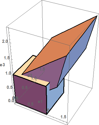
The deformation is very large as shown by applying this deformation to a unit cube (see figure below), so the strain measures are different.
The uniaxial small and Green strain along the vector  can be obtained as follows:
![\[ \varepsilon_{\mbox{small along }u}=\frac{u\cdot \varepsilon_{small}u}{\|u\|^2}=0.87\qquad \varepsilon_{\mbox{Green along }u}=\frac{u\cdot \varepsilon_{Green}u}{\|u\|^2}=1.31 \]](https://engcourses-uofa.ca/wp-content/ql-cache/quicklatex.com-309fb7576bc661574c81ae0cc58979b1_l3.png "Rendered by QuickLaTeX.com")
F={{1.2,0.2,0.2},{0.2,1.3,0.1},{0.9,0.5,1}};
X={X1,X2,X3};
x=F.X;
u=x-X;
Gradu=Table[D[u[[i]],X[[j]]],{i,1,3},{j,1,3}]
einfinitesimal=1/2*(Gradu+Transpose[Gradu]);
%//MatrixForm
egreen=1/2*(Gradu+Transpose[Gradu]+Transpose[Gradu].Gradu);
%//MatrixForm
u={1,1,1};
n=u/Norm[u];
n.einfinitesimal.n
n.egreen.n
Box1=Cuboid[{0,0,0},{1,1,1}];
Box2=GeometricTransformation[Box1,F];
Graphics3D[{EdgeForm[Thickness[0.01]],Box1,EdgeForm[Thickness[0.005]],Box2},Axes->True,AxesOrigin->{0,0,0},BaseStyle->Directive[Bold,15],AxesLabel->{e1,e2,e3}]
Example 2:
A cube of unit dimensions undergoes a rigid body rotation in  of
of  , then , and then
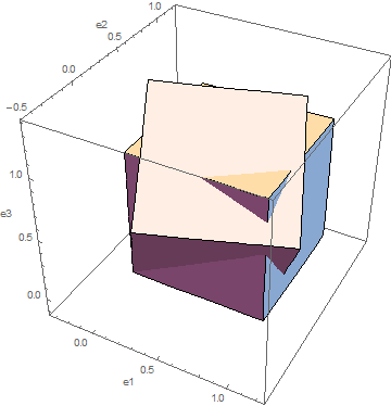
  around the basis vectors , , and respectively. Use Mathematica to visualize the box. Compare the two strain measures
  and .
and .
Solution:
The deformation gradient is given by:
![\[ F=Q_{e_1}Q_{e_2}Q_{e_3}=\left(\begin{matrix}0.883&-0.3214 & 0.3420\\0.4569&0.7553 & -0.4698\\-0.1073 & 0.5712 & 0.8138\end{matrix}\right) \]](https://engcourses-uofa.ca/wp-content/ql-cache/quicklatex.com-019e6d45ee99039409e41c05faf70517_l3.png "Rendered by QuickLaTeX.com")
Note that  is on the right since it is applied first.
The Green strain is identically zero while the small strain tensor predicts the following strains:
![\[ \varepsilon_{small}=\left(\begin{matrix}-0.117&0.068& 0.117\\0.068&-0.245 & 0.050\\0.117 & 0.051& -0.186\end{matrix}\right) \]](https://engcourses-uofa.ca/wp-content/ql-cache/quicklatex.com-a183f0471bcf851033919dfd567d93da_l3.png "Rendered by QuickLaTeX.com")
View Mathematica Code
Qx=RotationMatrix[thx,{1,0,0}];
Qy=RotationMatrix[thy,{0,1,0}];
Qz=RotationMatrix[thz,{0,0,1}];
thx=30Degree
thy=20Degree
thz=20Degree
F=Qx.Qy.Qz;
X={X1,X2,X3};
x=F.X;
u=x-X;
Gradu=Table[D[u[[i]],X[[j]]],{i,1,3},{j,1,3}];
einfinitesimal=1/2*(Gradu+Transpose[Gradu]);
einfinitesimal=FullSimplify[einfinitesimal];
%//MatrixForm
egreen=1/2*(Gradu+Transpose[Gradu]+Transpose[Gradu].Gradu);
egreen=FullSimplify[egreen];
%//MatrixForm
Box1=Cuboid[{0,0,0},{1,1,1}];
Box2=GeometricTransformation[Box1,F];
Graphics3D[{Box1,Box2},Axes->True,AxesOrigin->{0,0,},AxesLabel->{e1,e2,e3}]
Example 3:
A cube of unit length undergoes a simple shearing motion of an angle in the direction of and perpendicular to . Find the infinitesimal and Green strain measures that describe this motion. Comment on the difference between the two strain measures.
Solution:
The position function is given by:
![\[ x=\left(\begin{array}{c}x_1\\x_2\\x_3\end{array}\right)=\left(\begin{array}{c}X_1+\tan\theta X_2\\X_2\\X_3\end{array}\right) \]](https://engcourses-uofa.ca/wp-content/ql-cache/quicklatex.com-1e6e195372980aaa24f3b59689e737b9_l3.png "Rendered by QuickLaTeX.com")
The deformation gradient is given by:
![\[ F=\left(\begin{matrix}1&\tan\theta & 0\\0&1&0\\0&0&1\end{matrix}\right) \]](https://engcourses-uofa.ca/wp-content/ql-cache/quicklatex.com-7aa120722cb3f4a3562cb6122b729178_l3.png "Rendered by QuickLaTeX.com")
The small strain and Green strain tensors are given by:
![\[ \varepsilon_{small}=\left(\begin{matrix}0&\frac{\tan\theta}{2} & 0\\\frac{\tan\theta}{2}&0&0\\0&0&0\end{matrix}\right)\qquad \varepsilon_{Green}=\left(\begin{matrix}0&\frac{\tan\theta}{2} & 0\\\frac{\tan\theta}{2}&\frac{\tan^2\theta}{2}&0\\0&0&0\end{matrix}\right) \]](https://engcourses-uofa.ca/wp-content/ql-cache/quicklatex.com-d4588325ae684283c5f1518d57118a87_l3.png "Rendered by QuickLaTeX.com")
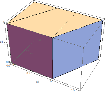
Both measures predict the same shear strains. For small deformations, both measures predict zero normal strains. As the increases, the vertical lines start developing large axial strains which the can predict while cannot. The undeformed and deformed shapes of the cube are shown below for  .
.
F={{1,Tan[theta],0},{0,1,0},{0,0,1}};
X={X1,X2,X3};
x=F.X;
u=x-X;
Gradu=Table[D[u[[i]],X[[j]]],{i,1,3},{j,1,3}]
einfinitesimal=1/2*(Gradu+Transpose[Gradu]);
einfinitesimal=FullSimplify[einfinitesimal];
%//MatrixForm
egreen= 1/2*(Gradu+Transpose[Gradu]+Transpose[Gradu].Gradu);
egreen=FullSimplify[egreen];
%//MatrixForm
Box1=Cuboid[{0,0,0},{1,1,1}];
Box2=GeometricTransformation[Box1,F];
theta=30Degree;
Graphics3D[{Box1,Box2},Axes->True,AxesOrigin->{0,0,0},AxesLabel->{e1,e2,e3}]
Example 4:
The following small strain matrix represents a two dimensional state of strain
![\[ \varepsilon_{small}=\left(\begin{matrix}0.01 & 0.012 \\ 0.012 & 0\end{matrix}\right) \]](https://engcourses-uofa.ca/wp-content/ql-cache/quicklatex.com-de22227f12b045f67b81f6651679d7c1_l3.png "Rendered by QuickLaTeX.com")
Find the principal strains and their directions. If a coordinate system is aligned with the principal directions, find the components of the strain matrix in this new coordinate system.
Solution:
The principal strains  and
and  and their directions
  , and
, and  be obtained using Mathematica by finding the eigenvalues and eigenvectors of . The following are the eiganvalues:
![\[ \varepsilon_1=0.018\qquad \varepsilon_2=-0.008 \]](https://engcourses-uofa.ca/wp-content/ql-cache/quicklatex.com-67ecf5373d7395f423589f9220e4fd54_l3.png "Rendered by QuickLaTeX.com")
The following are the normalized eigenvectors.
![\[ ev_1=\left(\begin{array}{c}0.83205\\0.5547\end{array}\right)\qquad ev_2=\left(\begin{array}{c}-0.5547\\0.83205\end{array}\right) \]](https://engcourses-uofa.ca/wp-content/ql-cache/quicklatex.com-a4c03ef88595578bbc4e7e3774f16600_l3.png "Rendered by QuickLaTeX.com")
The transformation matrix between the original coordinate system and the new coordinate system is:
![\[ Q=\left(\begin{matrix}0.83205 & 0.5547 \\ -0.5547 & 0.83205 \end{matrix}\right) \]](https://engcourses-uofa.ca/wp-content/ql-cache/quicklatex.com-8de67ff509241127ad88656618042f65_l3.png "Rendered by QuickLaTeX.com")
The strain matrix in the new coordinate system has the form:
![\[ \varepsilon'=Q\varepsilon Q^T=\left(\begin{matrix}0.018 & 0 \\ 0 & -0.008 \end{matrix}\right) \]](https://engcourses-uofa.ca/wp-content/ql-cache/quicklatex.com-2ba4818e9e682d07ad2071d0750d7b95_l3.png "Rendered by QuickLaTeX.com")
eps={{0.01,0.012},{0.012,0}};
s=Eigensystem[eps]
Q={-s[[2,1]],-s[[2,2]]}
epsdash=Chop[Q.eps.Transpose[Q]]
Example 5:
A state of uniform small strain is described by the following small strain matrix:
![\[ \varepsilon_{small}=\left(\begin{matrix}-0.01 & 0.002 & -0.023 \\ 0.002 & 0.05 & 0\\ -0.023 & 0 & 0.02\end{matrix}\right) \]](https://engcourses-uofa.ca/wp-content/ql-cache/quicklatex.com-c4ff302a731a713766d39fc62472c5e3_l3.png "Rendered by QuickLaTeX.com")
Determine the following:
- The longitudinal strain along the direction of the vector
 .
. - The change in the cosines of the angles between the vectors
 and
and  and comment on whether the angle between the vectors decreased or increased after deformation.
 - The shear strains of planes parallel to the vector
 and perpendicular to the vector
  .
.
Solution:
The strains along can be calculated as follows:
![\[ \varepsilon_{small \mbox{ along }dX}=\frac{dX\cdot\varepsilon_{small}dX}{\|dX\|^2}=0.0287 \]](https://engcourses-uofa.ca/wp-content/ql-cache/quicklatex.com-6ca7b2bec4f798b89da4f07a670d0eb9_l3.png "Rendered by QuickLaTeX.com")
The change in the cosines of the angles between the vectors and can be calculated as follows:
![\[ \frac{\cos\theta-\cos\Theta}{2}\simeq \frac{dX\cdot\varepsilon dY}{\|dX\|\|dY\|}=-0.0139 \]](https://engcourses-uofa.ca/wp-content/ql-cache/quicklatex.com-a6f5ced66c89d6e480e32fb78cc4cf9a_l3.png "Rendered by QuickLaTeX.com")
The angle between the vectors and before deformation can be calculated using the dot product:
![\[ \cos\Theta = \frac{dX\cdot dY}{\|dX\|\|dY\|}=\sqrt{\frac{2}{3}}\Rightarrow \Theta=0.6155rad=35.26^\circ \]](https://engcourses-uofa.ca/wp-content/ql-cache/quicklatex.com-0ac129aff0bf8db39fddf5177319b169_l3.png "Rendered by QuickLaTeX.com")
Therefore, the angle after deformation between the vectors is larger because:
![\[ \cos\theta-\sqrt{\frac{2}{3}}=-0.0248\Rightarrow \theta=0.662rad=37.93^\circ \]](https://engcourses-uofa.ca/wp-content/ql-cache/quicklatex.com-c5ebbbec2161b2eb7fb69a4d12390000_l3.png "Rendered by QuickLaTeX.com")
Since the vectors and are perpendicular, the shear strains of planes parallel to the vector and perpendicular to the vector can be obtained as follows:
![\[ \mbox{Shear strains of planes parallel to }dX\mbox{ and perpendicular to }dY=\frac{dX\cdot\varepsilon dY}{\|dX\|\|dY\|}=0.03rad \]](https://engcourses-uofa.ca/wp-content/ql-cache/quicklatex.com-7d652c20e8a2a14778282b251db02e10_l3.png "Rendered by QuickLaTeX.com")
Eps={{-0.01,0.002,-0.023},{0.002,0.05,0},{-0.023,0,0.02}};
dX={1,2,1};
Norm[dX]
Eps.dX
dX.Eps.dX/Norm[dX]^2
dX={1,0,1};
dY={1,1,1};
anglechange=dX.Eps.dY/Norm[dX]/Norm[dY]
THETA=N[ArcCos[dX.dY/Norm[dX]/Norm[dY]]]
THETA/Degree
theta=ArcCos[2*anglechange+Cos[THETA]]
theta/Degree
dX={-1,1,0};
dY={1,1,0};
ShearSTrain=dX.Eps.dY/Norm[dX]/Norm[dY]
Example 6:
The longitudinal engineering strains on the surface of a test specimen were measured using a strain gauge rosette to be 0.005, 0.002 and –0.001 along the three directions:  ,
,  , and
, and  respectively, where
  ,
,  , and
, and  . If the material is assumed to be in a small strain state, find the principal strains and their directions on the surface of the test specimen.
Solution:
The state of strain on the surface of the material can be represented by the symmetric small strain matrix:
![\[ \varepsilon_{small}=\left(\begin{matrix}\varepsilon_{11} & \varepsilon_{12} \\ \varepsilon_{12} & \varepsilon_{22}\end{matrix}\right) \]](https://engcourses-uofa.ca/wp-content/ql-cache/quicklatex.com-89821d0308b133837de49963d4dffc10_l3.png "Rendered by QuickLaTeX.com")
Since the longitudinal strain is known along three directions, three equations can be written to find the three unknown components of the strain matrix as follows:
![\[ \frac{a\cdot \varepsilon_{small}a}{\|a\|^2}=0.005 \qquad \frac{b\cdot \varepsilon_{small}b}{\|b\|^2}=0.002 \qquad \frac{c\cdot \varepsilon_{small}c}{\|c\|^2}=-0.001 \]](https://engcourses-uofa.ca/wp-content/ql-cache/quicklatex.com-b6e7a9b6c9b495b698cc2b506eeeb0d4_l3.png "Rendered by QuickLaTeX.com")
The norm of each of , , and is 1. Therefore, the three equations are:
![\[ \begin{split} \frac{1}{4}\left(3\varepsilon_{11}+2\sqrt{3}\varepsilon_{12}+\varepsilon_{22}\right) & = 0.005 \\ \varepsilon_{22}& = 0.002\\ \frac{1}{4}\left(3\varepsilon_{11}-2\sqrt{3}\varepsilon_{12}+\varepsilon_{22}\right) & = -0.001 \end{split} \]](https://engcourses-uofa.ca/wp-content/ql-cache/quicklatex.com-a44f153c433963f15a1453affda68dd3_l3.png "Rendered by QuickLaTeX.com")
Solving the above three equations yields:
![\[ \varepsilon_{small}=\left(\begin{matrix}\varepsilon_{11} & \varepsilon_{12} \\ \varepsilon_{12} & \varepsilon_{22}\end{matrix}\right)=\left(\begin{matrix}0.002 & 0.003464 \\ 0.003464 & 0.002\end{matrix}\right) \]](https://engcourses-uofa.ca/wp-content/ql-cache/quicklatex.com-0e4f66c28db95dde4ec7d74de4c3dd67_l3.png "Rendered by QuickLaTeX.com")
The principal strains and their directions are the eigenvalues and eigenvectors of the small strain matrix. The principal strains are:
![\[ \varepsilon_{1}=0.0055\qquad \varepsilon_2=-0.00146 \]](https://engcourses-uofa.ca/wp-content/ql-cache/quicklatex.com-118c2185613278c01f0764b1f7eaa657_l3.png "Rendered by QuickLaTeX.com")
The principal directions are:
![\[ ev_1=\left(\begin{array}{c}\frac{1}{\sqrt{2}}\\\frac{1}{\sqrt{2}}\end{array}\right)\qquad ev_2=\left(\begin{array}{c}\frac{-1}{\sqrt{2}}\\\frac{1}{\sqrt{2}}\end{array}\right) \]](https://engcourses-uofa.ca/wp-content/ql-cache/quicklatex.com-c1dfe0d0397d28e191b0675518cdc5da_l3.png "Rendered by QuickLaTeX.com")
eps=Table[Subscript[e,i,j],{i,1,2},{j,1,2}]
a={Cos[30Degree],Sin[30Degree]};
b={0,1};
c={-Cos[30Degree],Sin[30Degree]};
FullSimplify[a.eps.a/Norm[a]^2]
FullSimplify[b.eps.b/Norm[b]^2]
FullSimplify[c.eps.c/Norm[c]^2]
a=Solve[{a.eps.a/Norm[a]^2==0.005,b.eps.b/Norm[b]^2==0.002,c.eps.c/Norm[c]^2==-0.001,eps[[1,2]]==eps[[2,1]]},Flatten[eps]]
eps=eps/.a[[1]];
Eigensystem[eps]//MatrixForm
Example 7:
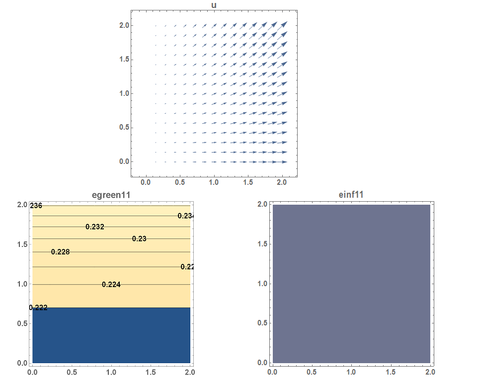
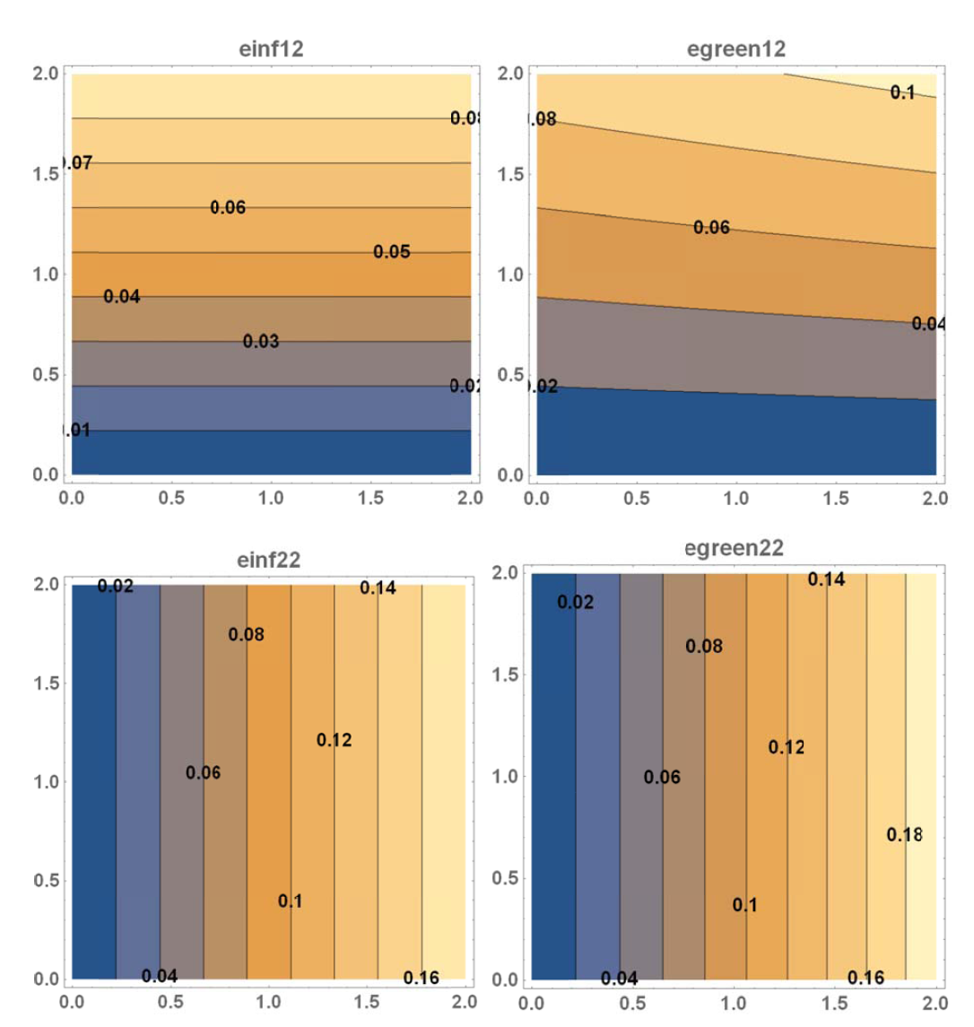
In the above examples, the deformation was described by a uniform strain matrix (i.e., a strain matrix that is not function in position). In this example, a nonuniform strain, i.e., the strain matrix is function of position is explored. Assume that the two dimensional displacement function of a 2units by 2units plate has the following form:
![\[ u=\left(\begin{array}{c}u_1\\u_2\end{array}\right)=\left(\begin{array}{c}0.2X_1\\0.09X_2X_1\end{array}\right) \]](https://engcourses-uofa.ca/wp-content/ql-cache/quicklatex.com-bff9dc36902f2bcf6432431379948c30_l3.png "Rendered by QuickLaTeX.com")
- Find the deformed configuration function
 .
. - Find and .
- Draw the vector plot of the displacement function on the plate.
- Draw the contour plots of
 ,
,  ,
,  , and
, and  on the plate.
Solution:
The position function of the deformed configuration is given by:
![\[ x=X+u=\left(\begin{array}{c}1.2X_1\\X_2+0.09X_2X_1\end{array}\right) \]](https://engcourses-uofa.ca/wp-content/ql-cache/quicklatex.com-6919b30b8bc0d8cda3ef187fe16abfc4_l3.png "Rendered by QuickLaTeX.com")
The deformation gradient is given by:
![\[ F=\left(\begin{matrix}1.2 & 0 \\0.09X_2 &1+ 0.09X_1\end{matrix}\right) \]](https://engcourses-uofa.ca/wp-content/ql-cache/quicklatex.com-e47df3d1ce5e07c5771a6eaef8358f2d_l3.png "Rendered by QuickLaTeX.com")
The displacement gradient is given by:
![\[ \nabla u=F-I=\left(\begin{matrix}0.2 & 0 \\0.09X_2 & 0.09X_1\end{matrix}\right) \]](https://engcourses-uofa.ca/wp-content/ql-cache/quicklatex.com-03561e5c9df24f7ad4c18cce9ce90e96_l3.png "Rendered by QuickLaTeX.com")
Therefore, the small strain matrix is given by:
![\[ \varepsilon_{small}=\left(\begin{matrix}0.2 & 0.045X_2 \\0.045X_2 & 0.09X_1\end{matrix}\right) \]](https://engcourses-uofa.ca/wp-content/ql-cache/quicklatex.com-b6a41b013dddd778ef42900dcfb8f1d2_l3.png "Rendered by QuickLaTeX.com")
The Green strain matrix is given by:
![\[ \varepsilon_{Green}=\left(\begin{matrix}0.22+0.00405X_2^2 & (0.045+0.00405X_1)X_2 \\(0.045+0.00405X_1)X_2 & (0.09+0.00405X_1)X_1\end{matrix}\right) \]](https://engcourses-uofa.ca/wp-content/ql-cache/quicklatex.com-d5eb0b4104aa360140580c55fdd3b176_l3.png "Rendered by QuickLaTeX.com")
The required plots are shown below.
View Mathematica Code
Clear[x1,x2,X1,X2]
X={X1,X2} ;
u={0.2X1,0.09X2*X1} ;
x=u+X;
Gradu=Table[D[u[[i]],X[[j]]],{i,1,2},{j,1,2}]
einfinitesimal=1/2*(Gradu+Transpose[Gradu]);
egreen=1/2*(Gradu+Transpose[Gradu]+Transpose[Gradu].Gradu);
einfinitesimal//MatrixForm
FullSimplify[egreen]//MatrixForm
VectorPlot[u,{X1,0,2},{X2,0,2},BaseStyle->Directive[Bold,15],AspectRatio->Automatic,PlotLabel->"u"]
ContourPlot[einfinitesimal[[1,1]],{X1,0,2},{X2,0,2} ,BaseStyle->Directive[Bold,15],AspectRatio->Automatic,ContourLabels->All,PlotLabel->"einf11"]
ContourPlot[egreen[[1,1]],{X1,0,2},{X2,0,2} ,BaseStyle->Directive[Bold,15],AspectRatio->Automatic,ContourLabels->All,PlotLabel->"egreen11"]
ContourPlot[einfinitesimal[[1,2]],{X1,0,2},{X2,0,2} ,BaseStyle->Directive[Bold,15],AspectRatio->Automatic,ContourLabels->All,PlotLabel->"einf12"]
ContourPlot[egreen[[1,2]],{X1,0,2},{X2,0,2} ,BaseStyle->Directive[Bold,15],AspectRatio->Automatic,ContourLabels->All,PlotLabel->"egreen12"]
ContourPlot[einfinitesimal[[2,2]],{X1,0,2},{X2,0,2} ,BaseStyle->Directive[Bold,15],AspectRatio->Automatic,ContourLabels->All,PlotLabel->"einf22"]
ContourPlot[egreen[[2,2]],{X1,0,2},{X2,0,2} ,BaseStyle->Directive[Bold,15],AspectRatio->Automatic,ContourLabels->All,PlotLabel->"egreen22"]
Problems:
- Which of the following functions describing motion is/are not physically possible and why?
-
 .
. -
 .
. -
 .
. -
 .
.
-
- Calculate the limits of
 and
and  for the following position functions to be physically possible:
-
 .
. -
 .
. -
 .
.
-
- Let a cube of unit length be represented by the set of vectors
 such that three of the cube’s sides are aligned with the three orthonormal basis set vectors , , and and one of the cube vertices lies on the origin of the coordinate system. Let
  be the deformed configuration such that
  is defined as :
![\[\begin{split} x_1&=1.1X_1+0.02X_1^2+0.01X_2+0.03X_3\\ x_2&=0.001X_1+0.9X_2+0.003X_3\\ x_3&=0.001X_1+0.005X_2+0.009X_3^2+0.9X_3 \end{split} \]](https://engcourses-uofa.ca/wp-content/ql-cache/quicklatex.com-8398d86a7f512ff612616f9e2308d0c7_l3.png "Rendered by QuickLaTeX.com")
Find the following:
- The displacement function .
- The new position of the 8 vertices of the cube.
- The deformed curves of the three edges of the cube that are aligned with the basis vectors , , and .
- The infinitesimal strain matrix and the volumetric strain as a function of the position inside the cube.
- The Green strain matrix as a function of the position inside the cube.
- Evaluate the infinitesimal strain matrix at two of the eight cube vertices.
- Evaluate the Green strain matrix at two of the eight cube vertices.
- The displacement function
- The reference and deformed configurations of an object exhibiting a two dimensional motion
 is shown in the figure below.
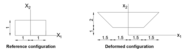
Find the following:- The two dimensional position function that can describe this shown motion.
- The associated two dimensional displacement function.
- The associated small strain tensor.
- The associated Green Lagrange strain tensor.
- A cube undergoes a deformation such that the infinitesimal strain is described by the matrix:
![\[ \varepsilon_{small}=\left(\begin{matrix}0.015&0.005&0\\0.005&-0.002&0\\0&0&0\end{matrix}\right) \]](https://engcourses-uofa.ca/wp-content/ql-cache/quicklatex.com-8dd3d6354ec7402821ee74609af36220_l3.png "Rendered by QuickLaTeX.com")
Find the following:
- The principal strains and their directions.
- The longitudinal strains along the direction of the vector:
![\[ dX=\left(\begin{array}{c}1\\1\\1\end{array}\right) \]](https://engcourses-uofa.ca/wp-content/ql-cache/quicklatex.com-c882c34e524fbeca56a9b22488f70676_l3.png "Rendered by QuickLaTeX.com")
- The approximate change in the angles between the vectors and
![\[ dY=\left(\begin{array}{c}-1\\1\\1\end{array}\right) \]](https://engcourses-uofa.ca/wp-content/ql-cache/quicklatex.com-53d24cda44c8899427d4824970c0a7ee_l3.png "Rendered by QuickLaTeX.com")
- The coordinate system transformation in which the strain matrix is diagonal. Express the strain matrix in the new coordinate system.
- The longitudinal engineering strains on the surface of a test specimen were measured using a strain rosette to be 0.005, 0.002, and –0.001 along the three directions: , , and
 where is along the direction of the basis vector , is oriented
  anticlockwise from , and is oriented anticlockwise from . If the material is assumed to be in a small strain state, find the principal strains and their directions on the surface of the test specimen.
 - The longitudinal engineering strains on the surface of a test specimen were measured using a strain rosette to be 0.006, -0.001, and 0.002 along the three directions: , , and where is along the direction of the basis vector , is oriented anticlockwise from , and is oriented anticlockwise from . If the material is assumed to be in a small strain state, find the principal strains and their directions on the surface of the test specimen.
- The measured strains for the three axes of a strain gauge rosette are:
 ,
,  , and
, and  . If coincides with the basis vector while and
  coincide with vectors that are anticlockwise and
  respectively from . Find the components of the strain tensor.
 - Assume that a two dimensional rectangular plate with dimensions 5 units along the basis vector and 1 unit along the basis vector is situated such that the origin of the coordinate system is at the midpoint of the left side of the plate. If the displacement function of the plate is described by:
![\[ \begin{split} u_1&=(-0.005X_1^2+0.004X_1)X_2\\ u_2&=-0.00016X_1^3+0.0012X_1^2\\ u_3&=0 \end{split} \]](https://engcourses-uofa.ca/wp-content/ql-cache/quicklatex.com-bfa3bce61d02889462976dfc1c5de0cf_l3.png "Rendered by QuickLaTeX.com")
find the following:
- The position function .
- The infinitesimal strain matrix as a function of the position.
- The Green strain matrix as a function of the position.
- Draw the vector plot of the displacement function.
- Draw the contour plots of , , , and .
- The position function
- Repeat the previous question if the displacement function is given by:
![\[ \begin{split} u_1&=(-0.001X_1^2+0.003X_1)X_2\\ u_2&=(-0.007X_2^2+0.003X_1^2)X_1\\ u_3&=0 \end{split} \]](https://engcourses-uofa.ca/wp-content/ql-cache/quicklatex.com-ba92e8e3b8d64b745245ecc3ec1cc418_l3.png "Rendered by QuickLaTeX.com")
- The general equation for the coordinates of a point
 on an ellipsoidal surface whose axes are oriented along the Cartesian coordinate system is:
![\[ \left(\frac{x_1}{a}\right)^2+\left(\frac{x_2}{b}\right)^2+\left(\frac{x_3}{c}\right)^2=1 \]](https://engcourses-uofa.ca/wp-content/ql-cache/quicklatex.com-acb3baf3e996c441ba9374ec2b77b26f_l3.png "Rendered by QuickLaTeX.com")
where
, , and are the three semi-diameters of the ellipsoidal surface. When  , the surface is a sphere with radius
  . Assuming that the motion of an object is described by the homogeneous deformation gradient
  such that the diagonal components of are the only non-zero components.
- Show that a sphere of radius deforms into an ellipsoid surface.
- Find the relationship between the semi-diameters of the ellipsoid and the components
 of the deformation gradient.
 - Find the relationship between the semi-diameters of the ellipsoid and the components
 of the infinitesimal strain tensor.
- Show that a sphere of radius
- Three unit square elements in
 deform as shown in the figure below.
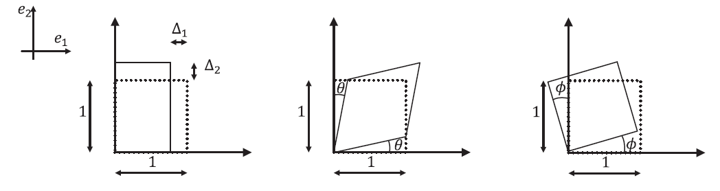
For each case:- Write expressions for the displacement components
 and
and  as functions of
  ,
,  , and the variables shown for each square.
 - Determine the components of the infinitesimal strain tensor and the infinitesimal rotation tensor.
- Determine the components of the Green strain tensor.
- Write expressions for the displacement components