Engineering at Alberta Courses » Mathematical Modelling of Plasticity

Plasticity: Mathematical Modelling of Plasticity

In this section, the physical behaviour described previously will be modelled theoretically. Most of the equations in this section were initially developed by “curve fitting” to the behaviour and thus, mathematical idealizations are considered to simplify the relationships. The classical mathematical modelling of plasticity is formulated “incrementally” as shown in the following sections.

Yield Stress and Codes of Practice:

The yielding and strain hardening regions of the metal stress strain curve shown in Figure 1 are characterized by an increase in the “yield stress” with an increase in the amount of plastic deformation. While some metals, for example mild steel, exhibit a distinct “yield stress”, others have a more round stress strain curve with a gradual decrease in the slope of the curve between the stress and the strain. The yield stress in general is history dependent, i.e., it depends on the history of loading of the specimen and is not a unique function of the current state of stress. Codes of practice often prescribe three specified minimum values for the properties of a steel to be fit for a specific application. These are normally the “yield stress” the “ultimate stress” and the “elongation” corresponding to the ultimate stress. The ultimate stress and the elongation corresponding to the ultimate stress can easily be obtained from any of the typical curves shown in Figure 2, however, obtaining the exact elastic limit could be practically very difficult, and therefore, codes of practice often define the “yield stress” to be the stress corresponding to a specific value of strain (e.g. 0.005) or to the stress corresponding to the intersection between the 0.002 offset of the linear stress strain portion (Figure 4). The two criteria do not necessarily predict the same value for the yield stress $\sigma_Y$ .

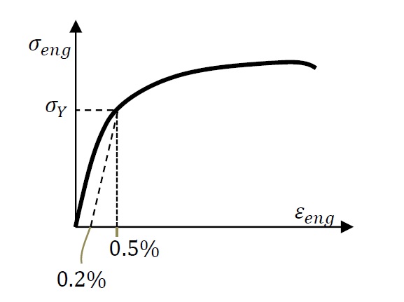
Figure 4. Definition of yield stress or $\sigma_Y$ given by different codes of practice

Stress Strain Idealization:

The relationship between the “true” stress versus the “true” or logarithmic strain is idealized to simplify the mathematical model. Points A and B are assumed to coincide and the loading and unloading in the yield and strain hardening region is assumed to follow a linear relationship as shown in Figure 5a. In other applications, especially those involving hand calculations or beam analysis, it is customary to assume an elastic-perfectly plastic stress strain curve, where the yield stress and the ultimate stress coincide (Figure 5b).

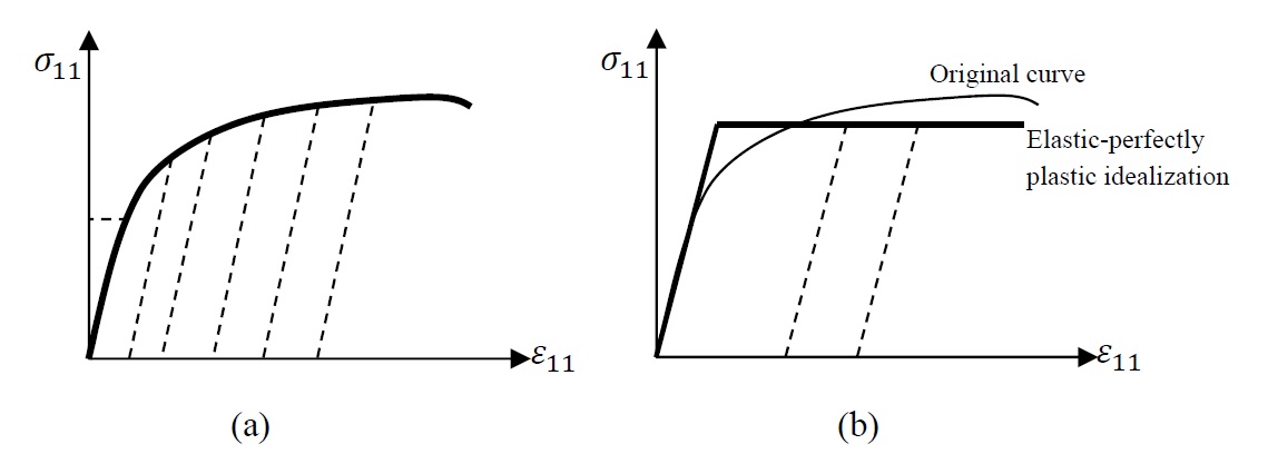
Figure 5. Different idealizations for the true stress versus true strain curves of metals: a) Unloading follows the dotted lines, b) elastic-perfectly plastic assumption with unloading following the dotted lines

Strain Decomposition and Incremental Behaviour in a Uniaxial Stress State:

Upon removal of the applied load, metals exhibit what is referred to as permanent or plastic deformation. The true longitudinal strain can thus be decomposed into two components: an elastic component corresponding to the applied stress, and a permanent plastic deformation. In a uniaxial stress state where the force is applied along the direction of the basis vector $e_1$ , $\sigma_{11}$ corresponds to the true stress or the Cauchy stress component and $\varepsilon_{11}$ corresponds to the true longitudinal strain or logarithmic longitudinal strain along the direction of the basis vector $e_1$ . The strain component can be decomposed into two components: an elastic component $\varepsilon_{11}^e$ and a plastic component $\varepsilon_{11}^p$ (Figure 6a). The elastic component is related to the stress using the linear elastic constitutive laws:

$\varepsilon_{11}^e=\frac{\sigma_{11}}{E}$

The plastic strain component can be obtained from the experimental results as follows:

$\varepsilon_{11}^p=\varepsilon_{11}-\frac{\sigma_{11}}{E}$

An explicit relationship describing the uniaxial stress component $\sigma_{11}$ and the plastic strain component $\varepsilon_{11}^p$ is often required (Figure 6b) for computations and thus a curve fitting model is often used. One of the very successful models is the Ramberg-Osgood model that fits a power law to the relationship between stress and plastic strain by introducing two material constants $k$ and $n$ as follows:

$\varepsilon_{11}^p=k\left(\frac{\sigma_{11}}{E}\right)^n$

If an increment in the load is such that $\sigma_{11}$ is decreased, then the elastic strain component is decreased while the plastic strain component stays the same. If an increment in the load is such that $\sigma_{11}$ reaches $\sigma_{Y}$ , then an increase beyond $\sigma_{Y}$ will cause an increase in the plastic strain $\varepsilon_{11}^p$ . i.e., unloading and reloading would follow vertical lines in Figure 6b. Thus, the above relationship in fact describes the magnitude of the yield stress at a certain value of a plastic strain parameter $\overline{\varepsilon^p}\in\mathbb{R}$ and is more precisely written in the form:

$\overline{\varepsilon^p}=k\left(\frac{\sigma_Y}{E}\right)^n$

The plastic strain parameter $\overline{\varepsilon^p}$ is a measure of the history of plastic deformation such that $\overline{\varepsilon^p}>0$ and is always increasing. The plastic strain parameter is also referred to as the equivalent plastic strain. The overbar is used to differentiate between the plastic strain parameter and the plastic strain tensor $\varepsilon^p\in\mathbb{M}^3$ .

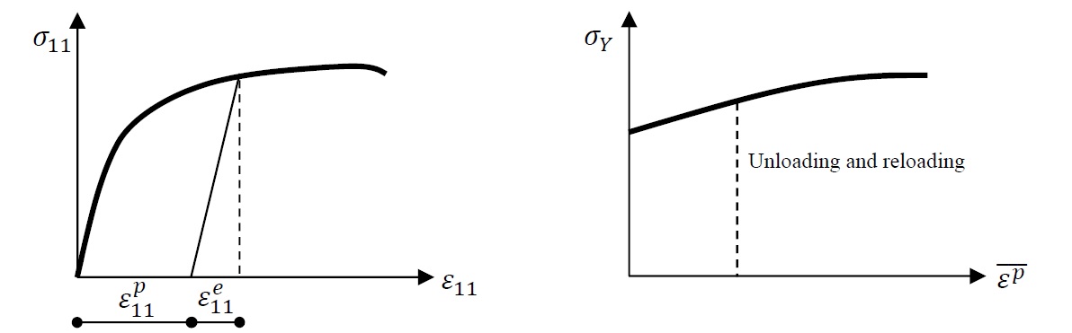
Figure 6. a) Decomposition of the strain component $\varepsilon_{11}$ into an elastic and a plastic component. b) the relationship between the plastic strain component and the applied stress

The remaining elastic strain components $\varepsilon_{22}^e, \varepsilon_{33}^e, \cdots$ can be obtained from the relationship between the stress and the strain. The remaining plastic strain components can be obtained from the isochoric deformation assumption and thus:

$\varepsilon_{22}^p=\varepsilon_{33}^p=-0.5\varepsilon_{11}^p$

In the above idealization, three functions were implicitly presented to fully describe the constitutive law of the plasticity of metals. These are the yield function, the hardening rule and the flow rule. As plastic deformation is dependent on the history of the loading, these functions can be conveniently written in terms of one parameter that represents the loading history. This one parameter is chosen to be the value of $\overline{\varepsilon^p}$ The following section describes these three rules.

Yield Function:

The yield function is the function that describes whether the material is about to exhibit plastic deformation or not. In a uniaxial state of stress, if $\sigma_{11}$ is less than $\sigma_{Y}$ then, the behaviour is elastic. Once $\sigma_{11}$ reaches $\sigma_{Y}$ then the material is about to exhibit plastic deformation. $\sigma_{11}$ can never be higher than $\sigma_{Y}$ since as $\sigma_{11}$ increases, $\sigma_{Y}$ increases as well. If the stress matrix of the uniaxial stress state is denoted by $\sigma$ , then the yield function can be defined as:

$f(\sigma)=\sigma_{11}-\sigma_{Y}\left(\overline{\varepsilon^p}\right)$

If $f(\sigma)<0$ , then the material is exhibiting elastic deformations, while if $f(\sigma)=0$ then, the material is about to exhibit plastic strain. As the material exhibits plastic strain, the change in the applied stress has to be such that the new stress state mathematically lies on the yield surface, i.e.,

$\dot{f}(\sigma)=\dot{\sigma}_{11}-\frac{d\sigma_Y}{d\overline{\varepsilon^p}}\dot{\overline{\varepsilon^p}}=0$

In other words, the rate of change of the stress components $\sigma_{11}$ is related to the rate of change of the equivalent plastic strain $\overline{\varepsilon^p}$ . The above relationship is called the consistency condition. Traditionally, the consistency condition is written in the following incremental form:

$\Delta f=\Delta \sigma_{11}-\Delta \sigma_Y=\Delta \sigma_{11}-\frac{d\sigma_Y}{d\overline{\varepsilon^p}}\Delta\overline{\varepsilon^p}=0$

The incremental form relates the increment in the increase in the applied stress to the incremental change of the yield stress of the material, or the increment in the applied stress to the increment in the plastic strain parameter. The incremental form represents a numerical integration scheme by which the increments in $\overline{\varepsilon^p}$ can be calculated as the applied stress is changed. The backward Euler numerical integration scheme is usually employed as it results in an approximation that is more accurate than the traditional forward Euler numerical integration scheme.

Hardening Rule:

The hardening rule is the function that gives the value of the yield stress as a function of the history of the loading. A typical relationship obtained from experiments is shown in Figure 6b and can conveniently be represented by the Ramberg-Osgood approximation:

$\overline{\varepsilon^p}=k\left(\frac{\sigma_Y}{E}\right)^n$

This relationship is termed the hardening rule. Given the current amount of the accumulated plastic strain parameter $\overline{\varepsilon^p}$ in the material, the value of the yield stress $\sigma_Y$ is obtained.

Flow Rule:

The flow rule is the function that dictates the amount of plastic strain that will accumulate during an increment in the loading. For a uniaxial state of stress the rate of change of the plastic strain aligned with the direction of the applied stress is equal to the rate of change of the plastic strain parameter (the equivalent plastic strain) $\dot{\varepsilon}_{11}^p=\dot{\overline{\varepsilon^p}}$ . The rate of change of the applied stress is equal to the rate of change of the yield stress, i.e,. $\dot{\sigma}_{11}=\dot{\sigma}_Y$ . Thus, the rates of change of $\varepsilon_{11}^p$ and $\sigma_{11}$ are related as follows:

$\dot{\varepsilon}_{11}^p=\frac{\dot{\sigma}_{11}}{\frac{d\sigma_Y}{d\overline{\varepsilon^p}}}$

In addition, the isochoric nature of the plastic deformation leads to the following relationship between the rates of change of the plastic strain components:

$\dot{\varepsilon}_{22}^p=\dot{\varepsilon}_{33}^p=-0.5\dot{\varepsilon}_{11}^p$

The above relationships can be written in incremental form such that $\Delta\varepsilon_{11}^p=\Delta\overline{\varepsilon^p}$ and $\Delta\sigma_{11}=\Delta\sigma_Y$ , then the increments in the plastic strain components are given by:

$\Delta\varepsilon_{11}^p=\frac{\Delta\sigma_{11}}{\frac{d\sigma_Y}{d\overline{\varepsilon^p}}}$

$\Delta\varepsilon_{22}^p=\Delta\varepsilon_{33}^p=-0.5\Delta\varepsilon_{11}^p$

The total value of the plastic strain components at the end of each increment is equal to the sum of all the plastic strain components increments developed throughout the loading. The backward Euler numerical integration scheme is usually employed for better accuracy.

Strain Decomposition and Incremental Behaviour in Multi-axial Stress States with Isotropic Hardening (No Bauschinger Effect):

The three functions that were presented in the previous section can be extended to cover a multi-axial stress state.

Multi-axial von Mises Yield Function:

The introduction of the multi-axial yield function dates back to the early years of the twentieth century with various researchers conducting experiments on the yielding of metals. As it was observed that metals are, in general, linear elastic isotropic materials and that yielding occurs independently of the hydrostatic stress, it was proposed that the material would start yielding once the deviatoric component of the elastic strain energy stored inside the material reaches a critical state. The expression for the deviatoric strain energy is equal to:

$\overline{U}_{deviatoric}=\frac{(von Mises stress)^2}{6G}$

Where, the von Mises stress, denoted by $\sigma_{vM}$ , is an invariant of the deviatoric stress tensor. The “critical” value at which the material starts to yield can be obtained from a uniaxial state of stress experiment. In the uniaxial state of stress, $\sigma_{vM}$ is equal to $\sigma_{11}$ and yielding will occur once $\sigma_{11}=\sigma_Y$ . Thus, the critical strain energy at the onset of yield is equal to:

$\overline{U}_{deviatoric critical}=\frac{\sigma_Y^2}{6G}$

Thus, in a state of stress described by a Cauchy stress matrix $\sigma$ , the yield function can be defined as follows:

$f(\sigma)=\sigma_{vM}-\sigma_Y$

In this relationship, $\sigma_{vM}$ describes the state of the stress inside the material while $\sigma_Y$ gives the maximum value that $\sigma_{vM}$ can attain before yielding. $\sigma_Y$ is presented as $\sigma_{max}$ in the stress based failure criteria section. Similar to the uniaxial case, if $f(\sigma)<0$ , then the material is exhibiting elastic deformations while if $f(\sigma)=0$ then, the material is about to exhibit plastic strain. The three dimensional version of the consistency condition presented above has the following form:

$\dot{f}(\sigma)=\sum_{i,j=1}^3\left(\frac{\partial \sigma_{vM}}{\partial \sigma_{ij}}\dot{\sigma}_{ij}\right)-\frac{d\sigma_Y}{d\overline{\varepsilon^p}}\dot{\overline{\varepsilon^p}}=0$

In other words, the rates of change of the stress components $\sigma_{ij}$ are related to the rate of change of the equivalent plastic strain $\overline{\varepsilon^p}$ . The incremental form of the consistency condition is such that $f(\sigma+\Delta\sigma)=0$ . This implies that as the stress changes, the yield function should not change and should also be equal to 0. Thus:

$\Delta f=\Delta\sigma_{vM}-\Delta\sigma_Y=\sum_{i,j=1}^3\left(\frac{\partial \sigma_{vM}}{\partial \sigma_{ij}}\Delta\sigma_{ij}\right)-\frac{d\sigma_Y}{d\overline{\varepsilon^p}}\Delta\overline{\varepsilon^p}=0$

The incremental form of the consistency condition in a multi-axial state of stress relates the increment in the increase in the applied stress represented by $\sigma_{vM}$ to the incremental change of the yield stress of the material, or the increment in the applied stress components $\Delta\sigma_{ij}$ to the increment in the accumulated plastic strain parameter $\Delta\overline{\varepsilon^p}$ . The backward Euler integration scheme is recommended for better accuracy of the results.

As shown in the stress based failure criteria section, if a coordinate system is chosen such that stress matrix is diagonal and the only possible nonzero components are $\sigma_1$ , $\sigma_2$ , and $\sigma_3$ , then the von Mises yield function is represented in the stress space by a cylinder whose axis is the line representing the hydrostatic stress states ( $\sigma_1=\sigma_2=\sigma_3$ ). To show this, we will investigate the the relationship:

$\left(\sigma_1-\sigma_2\right)^2+\left(\sigma_2-\sigma_3\right)^2+\left(\sigma_1-\sigma_3\right)^2=2\sigma_Y^2$

after a coordinate transformation into the new coordinate system $e'_1=\frac{1}{\sqrt{3}}\{1,1,1\}$ , $e'_2=\frac{1}{\sqrt{2}}\{1,-1,0\}$ , and $e'_3=\frac{1}{\sqrt{6}}\{1,1,-2\}$ . Obviously, $e'_1$ represents the line of the hydrostatic stress while $e'_2$ and $e'_3$ are perpendicular to that line. The coordinate transformation matrix into the new coordinate system has the form:

$Q=\left(\begin{matrix}\frac{1}{\sqrt{3}} & \frac{1}{\sqrt{3}} & \frac{1}{\sqrt{3}}\\ \frac{1}{\sqrt{2}} & \frac{-1}{\sqrt{2}} & 0\\ \frac{1}{\sqrt{6}} & \frac{1}{\sqrt{6}} & \frac{-2}{\sqrt{6}}\end{matrix}\right)$

A point with coordinates $\sigma=\{\sigma_1,\sigma_2,\sigma_3\}$ will have coordinates $a=\{a_1,a_2,a_3\}$ in the new coordinate system such that:

$\sigma=\left(\begin{array}{c}\sigma_1\\\sigma_2\\\sigma_3\end{array}\right)=Q^T \left(\begin{array}{c}a_1\\a_2\\a_3\end{array}\right)$

By replacing $\sigma_1$ , $\sigma_2$ , and $\sigma_3$ in the yield surface relationship with the coordinates $a_1$ , $a_2$ , and $a_3$ :

$a_2^2+a_3^2=\frac{2}{3}\sigma_Y^2$

Suggesting that in this new coordinate system, the relationship represents a cylinder whose axis is the vector $e'_1$ and whose radius is $\sqrt{\frac{2}{3}}\sigma_Y$ .
View Mathematica Code

Q = {{1/Sqrt[3], 1/Sqrt[3], 1/Sqrt[3]}, {1/Sqrt[2], -1/Sqrt[2], 0}, {1/Sqrt[6], 1/Sqrt[6], -2/Sqrt[6]}};
a = {a1, a2, a3};
s = Transpose[Q].a;
s // MatrixForm
FullSimplify[(s[[1]] - s[[2]])^2 + (s[[2]] - s[[3]])^2 + (s[[1]] - s[[3]])^2]

Another method to find the radius of the cylinder is by realizing that the stress state represented by the vector $oa$ in Figure 7 with the components $\sigma_1=\sigma_Y$ , $\sigma_2=\sigma_3=0$ lies on the surface of the cylinder. The unit vector representing the hydrostatic direction can be obtained by normalizing the vector $ob$ as follows:

$n=\frac{ob}{\|ob \|}=\frac{1}{\sqrt{3}} \left(\begin{array}{c} 1\\ 1\\ 1 \end{array} \right)$

The radius of the cylinder is given by the norm of the vector $ab$ as follows:

$\|ab\|=\|oa-(oa\cdot n)n\|=\left\|\left(\begin{array}{c}\sigma_Y\\0\\0\end{array}\right) - \frac{\sigma_Y}{3}\left(\begin{array}{c}1\\1\\1\end{array}\right)\right\|=\sqrt{\frac{2}{3}}\sigma_Y$

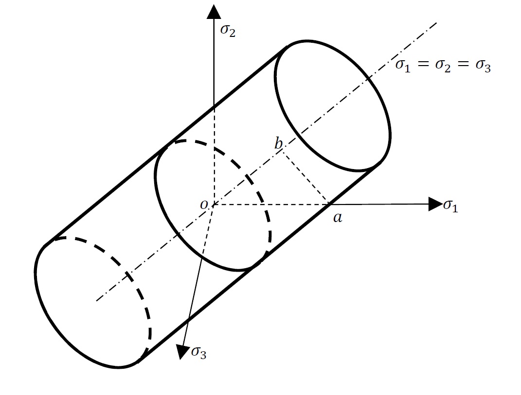
Figure 7. von Mises yield function in a multi-axial stress state represented in the stress space of the principal stresses

Multi-axial Tresca Yield Function:

Another yield function that predicts similar results is that given by the maximum shear stress as described in the stress based failure criteria section. The Tresca Yield function predicts that a material will yield when the maximum shear stress reaches a critical value $\tau_{max}$ :

$\frac{\max{\left(|\sigma_1-\sigma_2 |,|\sigma_1-\sigma_3 |,|\sigma_2-\sigma_3 |\right)}}{2}=\tau_{max}$

The “critical” value $\tau_{max}$ can be obtained from a uniaxial state of stress experiment. In the uniaxial state of stress, $\tau_{max}$ is equal to $\frac{\sigma_Y}{2}$ . Thus, in a state of stress described by a Cauchy stress matrix $\sigma$ , the Tresca yield function can be defined as follows:

$f(\sigma)=\max{\left(|\sigma_1-\sigma_2 |,|\sigma_1-\sigma_3 |,|\sigma_2-\sigma_3 |\right)}-\sigma_Y$

This yield function is represented graphically in the stress space of the principal stresses by a hexagon. Computational algorithms that use the von Mises yield criterion and those that use the Tresca yield criterion predict almost the same behaviour. While the von Mises yield criterion has a smoother curvature, the Tresca yield criterion may be easier for hand calculations. In general, when viewed on the plane perpendicular to the hydrostatic stress, the differences are practically negligible (Figure 8).

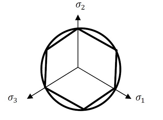
Figure 8. View perpendicular to the hydrostatic stress showing the difference between the von Mises (circle) and the Tresca (hexagon) yield surfaces.

Isotropic Hardening Rule:

In a multi-axial state of loading, the isotropic hardening rule predicts that the radius of the von Mises circle will change according to the relationship given between $\overline{\varepsilon^p}$ and $\sigma_Y$ . Usually, additional plastic strain (or plastic energy dissipation) applied to the material results in an increase in the radius of the von Mises circle (Figure 9).

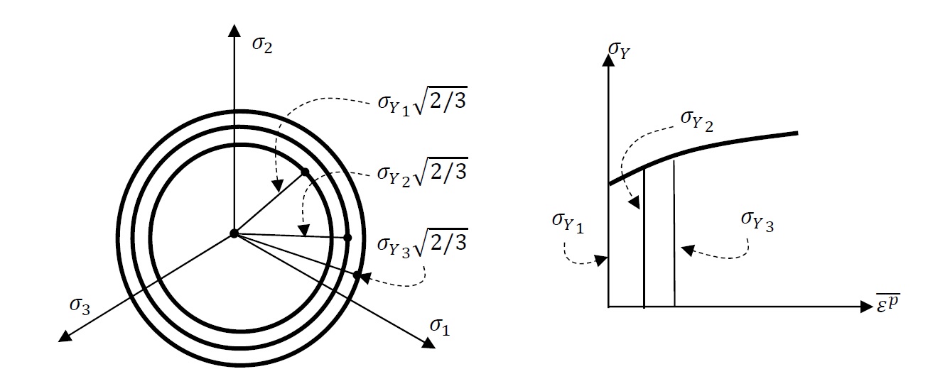
Figure 9. Isotropic hardening represented by a change (usually an increase) in the radius of the circle with the increase of the plastic strain parameter $\overline{\varepsilon^p}$

Multi-axial Flow Rule:

The last ingredient of incremental plasticity is to find the rate of change of the plastic strain components $\dot{\varepsilon}_{ij}^p$ associated with the rate of change of the stress components that is causing plastic flow. Experimental evidence suggest that the rates of the change of the plastic strain components are directly proportional to the applied deviatoric stress components as follows:

$\dot{\varepsilon}^p=\dot{\lambda}S\Rightarrow \dot{\varepsilon}_{ij}^p=\dot{\lambda}S_{ij}$

i.e.,

$\left( \begin{array}{ccc} \dot{\varepsilon}_{11}^p &\dot{\varepsilon}_{12}^p &\dot{\varepsilon}_{13}^p\\ \dot{\varepsilon}_{21}^p &\dot{\varepsilon}_{22}^p &\dot{\varepsilon}_{23}^p\\ \dot{\varepsilon}_{31}^p &\dot{\varepsilon}_{32}^p &\dot{\varepsilon}_{33}^p \end{array} \right)=\dot{\lambda} \left( \begin{array}{ccc} {S}_{11} &{S}_{12} &{S}_{13}\\ {S}_{21} &{S}_{22} &{S}_{23}\\ {S}_{31} &{S}_{32} &{S}_{33} \end{array} \right)$

The incremental form predicts that the increments in the plastic strain components are directly proportional to the deviatoric stress components in a material as follows:

$\Delta\varepsilon^p=\Delta\lambda S\Rightarrow \Delta\varepsilon_{ij}^p=\Delta\lambda S_{ij}$

i.e.,

$\left( \begin{array}{ccc} \Delta\varepsilon_{11}^p &\Delta\varepsilon_{12}^p &\Delta\varepsilon_{13}^p\\ \Delta\varepsilon_{21}^p &\Delta\varepsilon_{22}^p &\Delta\varepsilon_{23}^p\\ \Delta\varepsilon_{31}^p &\Delta\varepsilon_{32}^p &\Delta\varepsilon_{33}^p \end{array} \right)=\Delta\lambda \left( \begin{array}{ccc} {S}_{11} &{S}_{12} &{S}_{13}\\ {S}_{21} &{S}_{22} &{S}_{23}\\ {S}_{31} &{S}_{32} &{S}_{33} \end{array} \right)$

This observation conforms with the isochoric nature of the plastic deformation (why?). Notice that there is an inherent difference between the calculations of the plastic strain components and the elastic strain components. The increments of the elastic strain components are directly proportional to the increments in the stress components, while the plastic strain components, as observed from experiments, are directly proportional to the components of the deviatoric stress tensor.

In order to be able to compute the plastic strain components associated with a plastic flow instant, the constant of proportionality $\dot{\lambda}$ or $\Delta \lambda$ needs to be computed and then multiplied by the respective deviatoric stress component. This constant of proportionality can be obtained from energy considerations by assuming that the energy that goes into plastic deformation in a general state of stress is equal to the energy that goes into plastic deformation in a uniaxial state of stress. In a uniaxial state of the stress, the rate of the energy that is dissipated during the plastification of the material is equal to $\sigma_Y\dot{\overline{\varepsilon^p}}$ which is equal to $\sigma_{vM}\dot{\overline{\varepsilon^p}}$ . The energy dissipated during the plasticification of the material in a general state of stress is equal to $\sum_{i,j=1}^3 \left(\sigma_{ij}\dot{\varepsilon}_{ij}^p\right)$ . Assuming that the energy dissipated in the plastification process in a general state of stress is equal to that in a uniaxial state of stress results in the following:

$\sigma_{vM}\dot{\overline{\varepsilon^p}}=\sigma_{11}\dot{\varepsilon}_{11}^p+\sigma_{22}\dot{\varepsilon}_{22}^p+\sigma_{33}\dot{\varepsilon}_{33}^p+\sigma_{12}\dot{\varepsilon}_{12}^p+\sigma_{21}\dot{\varepsilon}_{21}^p+\sigma_{13}\dot{\varepsilon}_{13}^p+\sigma_{31}\dot{\varepsilon}_{31}^p+\sigma_{23}\dot{\varepsilon}_{23}^p+\sigma_{32}\dot{\varepsilon}_{32}^p$

Replacing the plastic strain components with the deviatoric stress components and the constant of proportionality $\dot{\lambda}$ results in the following expression:

$\sigma_{vM}\dot{\overline{\varepsilon^p}}=\dot{\lambda}\sum_{i,j=1}^3\sigma_{ij}S_{ij}$

However, since $\sigma_{ij}=S_{ij}+p\delta_{ij}$ and since $\sum_{i=1}^3S_{ii}=0$ , the stress components $\sigma_{ij}$ can be replaced with the deviatoric components as follows:

$\sigma_{vM}\dot{\overline{\varepsilon^p}}=\dot{\lambda}\sum_{i,j=1}^3S_{ij}S_{ij}$

Note that by definition, the von Mises stress is equal to:

$\sigma_{vM}=\sqrt{\frac{3}{2}\sum_{i,j=1}^3S_{ij}S_{ij}}$

Thus, the relationship between $\dot{\lambda}$ and $\dot{\overline{\varepsilon^p}}$ is as follows:

$\dot{\lambda}=\frac{\frac{3}{2}\dot{\overline{\varepsilon^p}}}{\sigma_{vM}}$

Therefore, the plastic strain components can be calculated by integrating the following differential equations functions in $\dot{\overline{\varepsilon^p}}$ :

$\dot{\varepsilon}_{ij}^p=\dot{\overline{\varepsilon^p}}\frac{3S_{ij}}{2\sigma_{vM}}$

The equivalent plastic strain is always positive and is a measure of the history of loading of the material. The term “equivalent plastic strain” is similar to the term “equivalent stress” that is used to denote $\sigma_{vM}$ . In addition, the rate of the “equivalent plastic strain” can be related to the rates of the plastic strain components with a relationship similar in form to that between $\sigma_{vM}$ and the deviatoric stress components:

$\sum_{i,j=1}^3\dot{\varepsilon}_{ij}^p\dot{\varepsilon}_{ij}^p=\sum_{i,j=1}^3\left(\frac{3}{2}\left(\dot{\overline{\varepsilon^p}}\right)^2 \frac{\frac{3}{2}S_{ij}S_{ij}}{\sigma_{vM}^2}\right)$

Therefore:

$\dot{\overline{\varepsilon^p}}=\sqrt{\frac{2}{3}\sum_{i,j=1}^3\dot{\varepsilon}_{ij}^p\dot{\varepsilon}_{ij}^p}$

The above relationship can be written in the following incremental form:

$\Delta\overline{\varepsilon^p}=\sqrt{\frac{2}{3}\sum_{i,j=1}^3\Delta\varepsilon_{ij}^p\Delta\varepsilon_{ij}^p}$

Associated Flow Rule:

The assumption that the incremental plastic strain components are directly proportional to the deviatoric stress components resulted in the final expression (as shown above):

$\dot{\varepsilon}_{ij}^p=\dot{\overline{\varepsilon^p}}\frac{3S_{ij}}{2\sigma_{vM}}$

It has been suggested in the early twentieth century that, similar to the existence of an “Elastic Potential Energy Function” from which the stress components and the elastic strain components are derived, the plastic strain components can also be derived from a “Plastic Potential Function” $\phi$ where:

$\dot{\varepsilon}_{ij}^p=\dot{\overline{\varepsilon^p}}\frac{\partial \phi}{\partial\sigma_{ij}}$

Careful investigation of the above expression in comparison with the previous expression for the incremental plastic strain components suggests that $\phi$ can be taken to be the yield function $\phi=f(\sigma)=\sigma_{vM}-\sigma_Y$ . In this case:

$\frac{\partial \phi}{\partial\sigma_{ij}}=\frac{\partial (\sigma_{vM}-\sigma_Y)}{\partial\sigma_{ij}}=\frac{\partial \sigma_{vM}}{\partial\sigma_{ij}}=\frac{3S_{ij}}{2\sigma_{vM}}$

Bonus Exercise: Show the following relation:

$\frac{\partial \sigma_{vM}}{\partial\sigma_{ij}}=\frac{3S_{ij}}{2\sigma_{vM}}$

The term “associated flow rule” is used to signify that the plastic strain components are derived from the yield function and thus, the flow rule is associated with the yield function. Associated flow rules are usually used for metal plasticity, while for plasticity of other materials, the incremental plastic strain components could be derived from different functions that are not associated with the yield function. In the latter case, the flow rule is termed: “non-associated flow rule”. Associated flow rules in metals that are derived from the von Mises or the Tresca yield surfaces predict zero volumetric plastic strain, however, in soils and many other materials, plasticity is associated with a change in volume and different “plastic potential” functions are utilized.

The Normality Rule:

Consider a smooth function $\phi:\mathbb{M}^3\rightarrow\mathbb{R}$ such that $\phi:\sigma\mapsto\mathbb{R}$ . With 9 independent components, $\sigma$ can also be viewed as an element of a 9 dimensional vector space. The function $\phi$ can then be considered as a smooth scalar valued function $\phi:\mathbb{R}^9\rightarrow\mathbb{R}$ . The gradient of $\phi$ with respect to its variables is denoted by $\nabla\phi$ and is defined as a vector field in $\mathbb{R}^9$ with components $\frac{\partial \phi}{\partial \sigma_{ij}}$ (See the section on the gradient of scalar fields). The direction pointing towards constant $\phi$ in $\mathbb{R}^9$ can be obtained as the unit vector $n$ along which the directional derivative is equal to zero:

$\nabla\phi\cdot n=0$

Thus, the vector $\nabla\phi$ is normal to the vectors pointing in the direction of constant $\phi$ . If $\phi$ is taken to be the yield function defined on the nine dimensional Euclidean vector space of the nine stress components (termed the stress space), then the vector $\nabla\phi$ is perpendicular to the direction of constant $\phi$ in the stress space. Since $\phi$ is constant ( $\phi=0$ ) on the yield surface, then $\nabla\phi$ is normal to the yield surface. The incremental plastic strain components can also be considered to be elements of a nine dimensional Euclidean vector space and the associated flow rule asserts that the nine dimensional vector $\Delta\varepsilon^p$ with components $\Delta\varepsilon_{ij}^p$ is linearly dependent on (parallel to) $\nabla\phi$ as:

$\Delta\varepsilon_{ij}^p=\Delta\overline{\varepsilon^p}\frac{\partial \phi}{\partial \sigma_{ij}}\Rightarrow \Delta\varepsilon^p=\Delta\overline{\varepsilon^p}\nabla\phi$

Thus, the nine dimensional vector $\Delta\varepsilon^p$ can also be viewed as normal (perpendicular) to the yield surface and thus, the associated flow rule leads to the normality rule. In a three dimensional vector space of the principal stresses of $\sigma$ , the components of $\Delta\varepsilon^p$ are perpendicular to the yield surface (Figure 10).
See Example 1 in the examples and exercises page for a detailed example of an isotropic hardening material model.

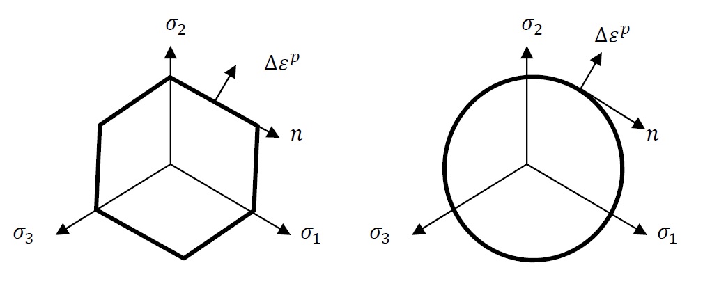
Figure 10. Schematic of the normality rule in the three dimensional vector space of the principal stresses.

Strain Decomposition and Incremental Behaviour in Multi-axial Stress State with Combined Kinematic and Isotropic Hardening (Bauschinger Effect):

In order to include the Bauschinger effect, various modifications to the isotropic hardening models presented in the previous section have been proposed throughout the development of the theory. The most successful and generalized form is that of the combined nonlinear kinematic and isotropic hardening model. In this section, the general form for this material model is presented.

Uniaxial Stress State Representation:

In a uniaxial state of stress, modelling the Bauschinger effect is implemented by assuming that the difference between the yield stress in tension and in compression is due to the shifting of the yield surface by a value that is equal to $\overline{\alpha}$ , which is termed the backstress. The yield stress $\sigma_Y$ is assumed to be the sum of two components: $\sigma_{Y\alpha}$ which is the yield stress with respect to the shifted centre of the yield surface and $\overline{\alpha}$ which describes the shifting of the yield surface. Both $\sigma_{Y\alpha}$ and $\overline{\alpha}$ are assumed to be functions of the history of the deformation represented by $\overline{\varepsilon^p}$ and the values of the stress increment. Figure 11 shows the schematics of three different models that can be utilized to model the Bauschinger effect. In the first model (Figure 11a), referred to as the linear kinematic model, the yield stress with respect to the shifted centre $\sigma_{Y\alpha}$ is assumed to be constant while the shifting of the centre of the yield surface is assumed to be linear. This model can be enhanced by assuming that the $\sigma_{Y\alpha}$ varies with the equivalent plastic strain in a nonlinear fashion (Figure 11b). It is also possible to assume that the backstress follows a nonlinear relationship leading to the general nonlinear combined kinematic and isotropic hardening model, as shown in Figure 11c. 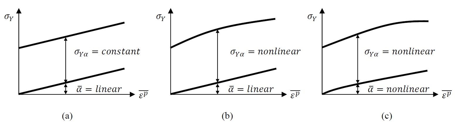Obviously, in order to calibrate such material model, numerous experiments have to be conducted to fit material curves for $\sigma_{Y\alpha}$ and for $\overline{\alpha}$ .

Figure 11. Three different models for the decomposition of the yield stress $\sigma_Y$ into a yield stress $\sigma_{Y\alpha}$ with respect to the centre of the yield surface and a backstress $\overline{\alpha}$ . (a) Kinematic hardening models, (b) combined linear kinematic hardening and nonlinear isotropic hardening model, (c) nonlinear kinematic and isotropic hardening model.

The most successful constitutive law model that describes the evolution of the backstress is the Armstrong-Frederick evolution law which in a uniaxial state of stress has the following form:

$\dot{\overline{\alpha}}=C\dot{\overline{\varepsilon^p}}-\gamma \overline{\alpha}\dot{\overline{\varepsilon^p}}$

or in incremental form:

$\Delta\overline{\alpha}=C\Delta\overline{\varepsilon^p}-\gamma \overline{\alpha}\Delta\overline{\varepsilon^p}$

Where $C$ and $\gamma$ are material constants. An earlier version of the above evolution law contained only the first term and was termed “Ziegler’s law”. Ziegler’s law had a limitation that $\overline{\alpha}$ would be unbounded and keeps increasing with the increase of the plastic strain $\varepsilon_{11}^p$ . The clever introduction of the term $\gamma \overline{\alpha}\dot{\overline{\varepsilon^p}}$ forces the value of $\overline{\alpha}$ to be bounded since integration of the above formula leads to:

$\int_0^{\overline{\alpha}} \! \frac{1}{C-\gamma\overline{\alpha}} \, \mathrm{d}\overline{\alpha}=\int_0^{\overline{\varepsilon^p}} \! \, \mathrm{d}\overline{\varepsilon^p}\Rightarrow \overline{\alpha}=\frac{C}{\gamma}(1-e^{-\gamma\overline{\varepsilon^p}})$

Thus, at higher levels of $\overline{\varepsilon^p}$ the value of $\overline{\alpha}$ is bounded by the ratio of the material constants $\frac{C}{\gamma}$ .

Multi-axial Stress State Implementation:

In order to implement the above relationships in a multi-axial stress state, the backstress is assumed to be a tensor $\alpha\in\mathbb{M}^3$ with components $\alpha_{ij}$ . The yield function in this case is given as follows:

$f(\sigma-\alpha)=\sigma_{vM}|_{\sigma-\alpha}-\sigma_{Y\alpha}$

where $\sigma_{vM}|_{\sigma-\alpha}$ is the von Mises stress but with the difference $\sigma-\alpha$ substituted instead of the stress tensor $\sigma$ . Figure 12 shows the graphical representation of the yield function in the stress space of the principal stresses. If $\alpha^{dev}\in\mathbb{M}^3$ is the deviatoric backstress tensor, then, the yield function can be written as:

$f(\sigma-\alpha)=\sqrt{\sum_{i,j=1}^3\frac{3}{2}(S_{ij}-\alpha_{ij}^{dev})(S_{ij}-\alpha_{ij}^{dev})}-\sigma_{Y\alpha}$

The Armstrong-Frederick material model describing the evolution of the backstress in a multi-axial stress state is given by the following form:

$\dot{\alpha}_{ij}=\left(\frac{C(\sigma_{ij}-\alpha_{ij})}{\sigma_{Y\alpha}}-\gamma \alpha_{ij}\right)\dot{\overline{\varepsilon^p}}$

Or in incremental form:

$\Delta\alpha_{ij}=\left(\frac{C(\sigma_{ij}-\alpha_{ij})}{\sigma_{Y\alpha}}-\gamma \alpha_{ij}\right)\Delta\overline{\varepsilon^p}$

The bounding limit of $\alpha_{ij}$ is given by the value $\frac{C}{\gamma}$ and thus, the centre of the yield surface in the stress space is bounded by a cylinder of radius $\sqrt{\frac{2}{3}}\frac{C}{\gamma}$ , while the yield surface is bounded by the cylinder with a radius equal to $\sqrt{\frac{2}{3}}\sigma_{max}$ (Figure 12).

The associated flow rule can still be used for this material model where the plastic strain components are calculated as follows:

$\dot{\varepsilon}_{ij}^p=\dot{\overline{\varepsilon^p}}\frac{\partial \phi}{\partial\sigma_{ij}}=\dot{\overline{\varepsilon^p}}\left(\frac{\frac{3}{2}(S_{ij}-\alpha_{ij}^{dev})}{\sigma_{vM}|_{\sigma-\alpha}}\right)$

Or in incremental form:

$\Delta\varepsilon_{ij}^p=\Delta\overline{\varepsilon^p}\frac{\partial \phi}{\partial\sigma_{ij}}=\Delta\overline{\varepsilon^p}\left(\frac{\frac{3}{2}(S_{ij}-\alpha_{ij}^{dev})}{\sigma_{vM}|_{\sigma-\alpha}}\right)$

The increment in the plastic strain parameter can be obtained from the consistency condition as follows:

$\dot{f}=\sum_{i,j=1}^3\frac{\partial f}{\partial \sigma_{ij}}\dot{\sigma}_{ij}+\sum_{i,j=1}^3\frac{\partial f}{\partial \alpha_{ij}}\dot{\alpha}_{ij}-\frac{d\sigma_{Y\alpha}}{d\overline{\varepsilon^p}}\dot{\overline{\varepsilon^p}}=0$

or in incremental form:

$\Delta f=\sum_{i,j=1}^3\frac{\partial f}{\partial \sigma_{ij}}\Delta\sigma_{ij}+\sum_{i,j=1}^3\frac{\partial f}{\partial \alpha_{ij}}\Delta\alpha_{ij}-\frac{d\sigma_{Y\alpha}}{d\overline{\varepsilon^p}}\Delta\overline{\varepsilon^p}=0$

With

$\frac{\partial f}{\partial \sigma_{ij}}=-\frac{\partial f}{\partial \alpha_{ij}}=\frac{\frac{3}{2}(S_{ij}-\alpha_{ij}^{dev})}{\sigma_{vM}|_{\sigma-\alpha}}$

Bonus exercise:
Deduce the above relationship for $\frac{\partial f}{\partial \sigma_{ij}}$

See Example 2 in the examples and exercises page for a detailed example of a nonlinear kinematic hardening material model.

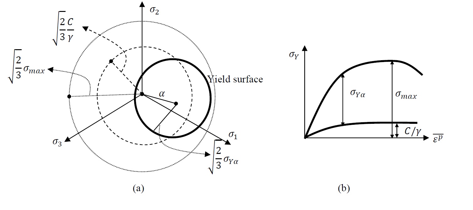
Figure 12. (a) Schematic showing the shifted yield surface in the three dimensional stress space of the principal stresses. The inner dotted circle represents the bounding limits of the centre of the yield surface, while the outer dotted circle represents the bounding limits of the maximum stress. (b) Uniaxial representation

Open Educational Resources