
Engineering Mechanics: STATICS: Scalars and vectors
Basic definitions
Scalars and vectors are mathematical objects and they are useful for quantifying physical quantities.
Scalar. A scalar is a real number. For example  ,
,  ,
,  ,
,  , and so on .
Scalar quantity. A scalar quantity is a quantity that can be described by a single real number. This number specifies the magnitude or size of that quantity. For example mass, speed, area, temperature, and pressure are scalar quantities.
Sometimes a scalar quantity is simply referred to as scalar. For example, “mass is a scalar” is equivalent to stating: “mass is a scalar quantity”.
Mathematical operations on scalars follow the usual rules of arithmetic.
Vector. A vector is a mathematical object that is understood by its size (magnitude) and its direction. This definition perfectly fulfils the requirements of engineering mechanics. However, for a more rigorous mathematical definition, please refer to section 14.2.8.
Vector quantity. A vector quantity is a quantity characterized by both a magnitude and a direction. For example velocity, force, acceleration, and moment are all vector quantities.
The magnitude (sometimes referred to as the norm) of a vector is always taken to be a positive number. For example the magnitude of the velocity of a moving object is the speed of that object. Speed is always measured and reported as a positive number.
The terms vector and vector quantity can be equivalently used.
In this book, we distinguish between a vector and a scalar using special notations. The notation for a vector is a bold upper-case letter  or an upper-case letter with a symbolic overhead arrow
  . By convention, the direction of the arrow is from left to right and it does not convey any information about the direction of the vector itself. The magnitude of a vector is denoted by a regular upper-case letter
  or the vector notation embedded by two vertical lines
  or
or  . The embedding vertical line notation is also used to denote the absolute value of a scalar, for example
  where
where  is a real number. In some text the notation of vector magnitude is a double-vertical-line notation
  and the absolute value of a scalar is shown by . In this book,
  is used for both cases.
Using an upper-case letter with a symbolic overhead arrow is recommended when writing notes, assignments, or exams.
Graphical representation of vectors
A graphical or geometrical representation of vectors is by directed line segments or arrows. Actually, a directed line segment is a vector itself.
A line segment is a finite-length piece of a straight line. It is defined by two ending points on a straight line.
A directed line segment (arrow) is a line segment with a defined direction. To define the direction, one of the segment’s end point is distinguished as the tail, and consequently the other one as head. Thereby, the r direction is defined as the sense of direction from the tail to the head of the segment. A directed line segment can be displayed by an arrow such that the arrow head defines the sense of direction. The line that is coincident with an arrow is called the line of action. The orientation or direction of an arrow (its tail is already known or defined) with respect to a fixed axis (a line) is defined by an angle formed between the axis and the line of action of the arrow. Figure 1 shows a directed line segment or arrow representing the vector  with its defined terms.
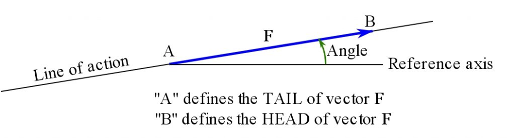
Figure 1. Geometric representation of a directed line segment (arrow) or a vector.
A directed line segment or simply an arrow has both the direction and length. The length of an arrow is defined as its magnitude. An arrow has both a direction and a magnitude, therefore, an arrow is a vector. To be more precise an arrow is a geometric vector. In this book, vectors and arrow are equivalent.
Zero vector. The zero vector, denoted by  or
or  , is a vector of length zero. The zero vector does not point toward any direction, therefore, its direction is undefined.
An important remark with a vector is that the position of a directed line segment or a vector in the space does not change the properties of the vector; because a vector is defined only by its direction and magnitude. As a result, two vectors are equal if they have the same direction and magnitude. Examples of equal vectors are shown in Figure 2 below.

Figure 2. Equivalent vectors.
Vector operations using the parallelogram rule and trigonometry
The following are mathematical operations defined on vectors:
- Multiplication (or division) by a scalar.
- Vector addition (or subtraction).
- Vector products (dot product and cross product).
The first two operations are the fundamental operations. Vector products are special functions on vectors discussed in sections 14.2.6 and 14.27. In this section, the first two operations are discussed.
Multiplication (and division) of a vector by a scalar
A vector can be multiplied by a scalar and the result is another vector. A vector  multiplied by a scalar
  will be equal the vector
  . This operation is denoted by
  . Division of a vector by a scalar
  is the same as multiplication by
  . Multiplication of a vector by a scalar is implemented by this rule:
Scalar multiplication simply scales the magnitude (length) of a vector if the scalar is a positive number. The operation also reverses the direction of the vector if the scalar is a negative number.
The following figure demonstrates different vectors as the results of multiplication of by a scalar.
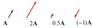
Figure 3. Multiplication of a vector by a scalar.
, if  then
then  scales and reverse (switches) the direction of .
Remark: multiplication of any vector, , by zero results in the zero vector:  .
.
Remark: multiplying a vector by a scalar scales its magnitude: if , then  in which
  is the absolute value of the scalar .
Colinear vectors. Vectors on the same straight line are called colinear vectors. In other word, and are colinear if and only if there is an scalar such that  . If
. If  then the absolute value of is
  , because
  . According to this definition, the zero vector is colinear with all other vectors.
It should be noted that parallel arrows or parallel vectors (vectors with parallel lines of action) are colinear because they can be moved on the same straight line.
Concurrent vectors. Vectors with their tails starting at the same point are called concurrent. This definition is only for the sake of graphical representation of arrows as vectors. Any number of vector can become concurrent once they are moved (re-drawn) such chat they all start from the same point.
Unit vector. A unit vector is a vector of magnitude  . Any vector can be written as a scalar multiplication of a unit vector with the same direction:
  such that the notation
  indicates the unit vector (
 ) in the direction of . Any vector
  can become a unit vector if scaled by
  . In this case we write
  and call the unit vector of . Obviously, is colinear with .
Normalizing a vector. Making a unit vector out of a vector is called normalizing a vector. The resultant unit vector only shows the direction of the original vector.
Vector addition
Vector addition is a vector operation that produces another vector. The addition of two vectors and resulting in a vector  is denoted as:
  . There are two equivalent rules (laws) for vector addition: triangle rule, and parallelogram law.
To calculate using the triangle rule follow these steps:
- Put and head to tail (or tail to head), and then,
- Close the triangle with the vector .
Figure 4 demonstrates the triangle rule for vector addition.
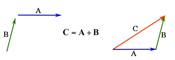
Figure 4. Addition of two vectors by The triangle rule.
 . This can be readily observed in the following figure:
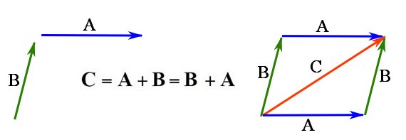
Figure 5. Commutative property of vector addition.
leads to the parallelogram law. To add two vectors using the parallelogram law, follow these steps:
- Bring the vectors to join at a point, say
 , by their tails (make the vectors concurrent).
 - From the head of each vector draw a line parallel to the other vector. These two lines intersect at a point
 and form two adjacent lines of a parallelogram.
 - Draw a vector on the diagonal of the parallelogram from point to the point . This vector is the resultant vector
 .
.
The figure below demonstrates vector addition using the parallelogram law.
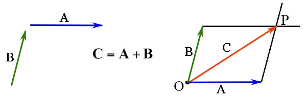
Figure 6. The parallelogram law.
and the operation  can be written as
  which means adding to with its direction revered. An example is shown in Figure 7.
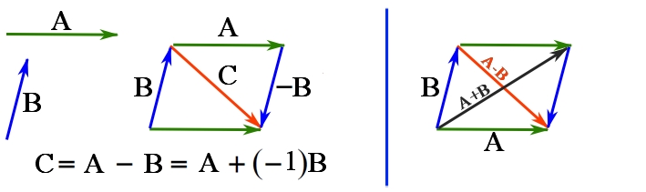
Figure 7. Vector subtraction.
Remark: while vector addition is commutative ( , vector subtraction is not commutative because
  . In fact,
  .
.
Addition of colinear vectors. The addition of colinear vectors are naturally handled by the triangle rule. Examples of vector addition in the case of colinear vectors are demonstrated in Figure 8.
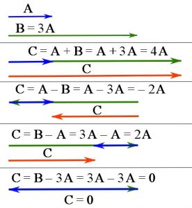
Figure 8. Vector addition of parallel or colinear vectors.
 . An example is as demonstrated below:

Figure 9. Successive addition of 3 vectors using the triangle rule.
Trigonometry for vector operations
The triangle and parallelogram rules graphically give the resultant vector such that the direction of the vector can be understood. To calculate the magnitude of the resultant vector and the angle it makes with other vectors, trigonometry laws are used. Basic trigonometry laws are:

Figure 10. Basic trigonometry laws.

Figure 11. Sine and Cosine Laws.
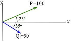
Example 1
Determine the magnitude of the resultant vector  and its direction measured counterclockwise from the positive x-axis shown.
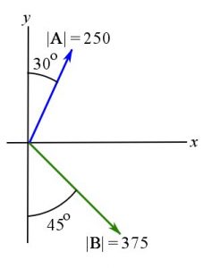
Solution
— to be added —
Remark: It should be understood that the magnitude of vector addition is not necessarily equal the addition of the magnitudes. In other words,  . In fact,
  always holds. This statement, called the triangle inequality, can be explored or proved by using the Cosine law.
Vector components and Cartesian vector notation
The vector operation  can be considered as decomposing the vector into two vector components
  and
and  . This implies that has two components along the directions or lines of action of and (Figure 12). Given a set of directions, a component of a vector along each directions can be found by decomposing the vectors. Vector decomposition of can be regarded as the reverse of the vector addition, which means finding vectors with known directions (but unknown magnitude) such that their addition equals . Decomposing a vector can be performed using the trigonometry laws.
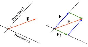
Figure 12. Decomposing a (planar) vector into two components along two directions or lines.
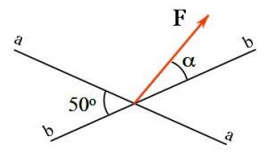
Example 2
The vector of magnitude  is to be resolved into two components along the lines a-a and b-b. Determine the angle
  if the component of along the line a-a has a magnitude of
  , i.e.
  .
.
Solution
— to be added —
Vector decomposition makes the resultant vector components on each direction collinear. This makes the addition of the vector components on a particular direction straight forward.
Example 3
Determine the resultant vector,  , by decomposing the vectors
  and
and  on the two perpendicular lines (axes) denoted by
  and
and  .
.
Solution
— to be added —
In the above example, the vectors are resolved into their components on the given axes and the collinear components of the vectors are added. Then, adding the resultant vectors on the axes gives the final resultant vector. This approach is a systematic approach for adding vectors.
Adding more than two vectors through a direct use of the parallelogram law, the Sine and Cosine laws is cumbersome. To do vector addition efficiently and in a systematic way, vectors are to be decomposed (resolved) onto a set of directions and the vector addition is performed using the colinear components.
In this regard, a set of directions simplifying the equations should be chosen. A convenient set of directions is a set of perpendicular directions called orthogonal axes. Orthogonal means perpendicular and an axis is a line to which a positive direction is associated by a vector colinear with the line. The positive direction of an axis sets a benchmark determining the positive (or negative) directions of the colinear vectors with the axis. For example, considering an axis shown in Figure 13, we say is in the positive direction and is in the negative direction (with respect to the positive direction defined by the axis).

Figure 13. Definition of an axis.
A vector decomposed (resolved) into its rectangular components can be expressed by using two possible notations namely the scalar notation (components) and the Cartesian vector notation. Both notations are explained for the planar conditions, and then expanded to three dimensions.
Rectangular vector components of coplanar vectors
Consider a vector and its rectangular components resolved in a Cartesian system as shown in Figure 14. The and vector components of are resolved and denoted by  and
and  respectively. The subscripts and denote the axes with which the components are colinear. The magnitude of the vector components are
  and
and  . By the definition the magnitude of the vectors are (has to be) positive. Therefore, the magnitude of the components does not have information about their directions. To include the information about the directions of the vector components in a Cartesian system, scalar notation or scalar components are defined. Scalar components of a vector are signed magnitudes of its rectangular components. A scalar component is positive if the vector component is directed along the positive axis, and negative if the vector component is directed along the negative axis (opposite of the axis positive direction). For the vector components and shown in Figure 14, the scalar components are denoted by
  and
and  . Note the regular and italic font face used for the notation. The scalar components of the vector shown in Figure 14a are
  and
and  both being positive. The scalar components of the vector shown in Figure 14b, however, are and
  . The scalar component is negative, because its vector component is directed along the negative direction of the axis.
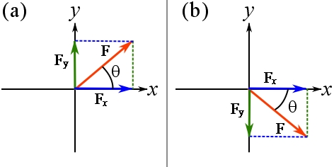
Figure 14. Components of vectors resolved in the Cartesian system.
 . The first element indicated the component and the second one refers to the component. The scalar components of a vector are also referred to as the coordinates of a vector.
By the definition (Figure 13), an axis has an associated vector showing the positive direction of the axis. Conventionally, the vector associated with an axis is considered to be a unit vector. Any vector on an axis (or parallel with the axis) is colinear with the unit vector of an axis. Therefore, any vector on an axis can be written as an scalar multiplier of the axis unit vector. The scalar multiplier is equal to the signed magnitude of the vector on the axis. It is positive if the vector is in the direction of the axis unit vector, and negative otherwise.
The unit vectors associated with the Cartesian and axes are denoted by bold small letters  and
and  respectively and their respective small arrows are displayed on or near the Cartesian axes (Figure 15). Another possible notations are
  and
and  .
.
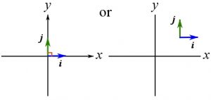
Figure 15. The planar Cartesian axes and their unit vectors.
can be now expressed in terms of the Cartesian axis unit vectors:  . The notation
  or
or  is used for any vector component is in the opposite direction of its axis unit vector. For example, the vector on Figure 14.b is resolved to its rectangular components as:
  .
.
As a general rule any vector can be written as  in a Cartesian system. The notation
  means any of the signs are independently possible. Showing a vector by the addition of its rectangular components expressed in terms of the unit vectors and is called the Cartesian vector notation (CVN).
Remark: Both the scalar notation and the CVN are equivalent by noting that  .
.
Remark: using the CVN is equivalent to resolving a vector in the Cartesian coordinate system.
Remark: components of a vector, referring to the vector components, are vectors, whereas, the scalar components, also known as the coordinates of a vector, are scalar.
Example 4
Determine the rectangular components of (shown in the figure below) and write them in both the scalar notation and CVN.
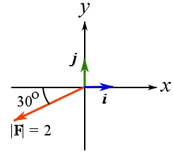
Solution
— to be added —
Remark: the apparent location of a vector on a plane does not affect its component. You can always consider (draw) the Cartesian axes at the tail of a vector and calculate its components.
It is worthy to note the relationships among the scalar components, the magnitude, and the direction of a vector. Consider a Cartesian coordinate system in which angles are measured counter clockwise from the axis as demonstrated in Figure 16. Then the following equations hold:
(1) ![\[ \begin{split}F^2&=\vert \bold F\vert^2 =F_x^2 + F_y^2 \quad \text{or}\quad F=\vert \bold F\vert =\sqrt {F_x^2 + F_y^2}\\ \tan \theta &= \frac{F_y}{F_x},\quad \sin\theta=\frac{F_y}{F},\quad\cos\theta=\frac{F_x}{F}\quad\text{for }0^\circ\le \theta < 360^\circ \end{split}\]](https://engcourses-uofa.ca/wp-content/ql-cache/quicklatex.com-e652ce915f3b813eccd8b905397b44eb_l3.png "Rendered by QuickLaTeX.com")
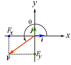
Figure 16. The relationship between the scalar components of a vector and its magnitude, and direction.
 and consequently the absolute values of the scalar components (which are the magnitudes of the vector components) should be used in the trigonometry Laws. Figure 17a demonstrates some examples. Another way of specifying the direction of a planar vector is by a small slope triangle. The small slope triangle conveys the information on
  ,
,  , and
, and  of the acute angle that the vector makes with an axis (Figure 17b).

Figure 17. Specifying the direction of a planar vector in the Cartesian frame by the acute angle that the vector makes with any of the Cartesian axes.
(2) ![\[\begin{split} F^2&=\vert \bold F\vert^2 =F_x^2 + F_y^2 \quad \text{or}\quad F=\vert \bold F\vert =\sqrt {F_x^2 + F_y^2} \\ \tan \theta &= \frac{\mid F_y\mid}{\mid F_x\mid},\quad \sin\theta=\frac{\mid F_y\mid}{F},\quad\cos\theta=\frac{\mid F_x\mid}{F}\quad\text{for }0^\circ\le \theta < 90^\circ \end{split}\]](https://engcourses-uofa.ca/wp-content/ql-cache/quicklatex.com-65a327b9271d775c7fa33aac812d0046_l3.png "Rendered by QuickLaTeX.com")
Remark: be cautious about the way the direction of a vector is specified and the proper formulation you should use for the calculations. If an acute angle is used, you should determine the signs of the scalar components by observing the direction of the vector components.
Remark: using an acute angle to specify the direction of an vector has a calculation advantage that  is in the domain of the inverse trigonometric functions
  ,
,  and
and  .
.
Planar vector operations using CVN (two dimensions)
Addition of several vectors  using the CVN takes the following steps:
1- Express each vector in CVN by resolving the vector to its rectangular components:
![\[\begin{split} \bold F_1&=F_{1x}\bold i + F_{1y}\bold j\\ \bold F_2&=F_{2x}\bold i + F_{2y}\bold j\\ &\vdots\\ \bold F_n&=F_{nx}\bold i + F_{ny}\bold j \end{split} \]](https://engcourses-uofa.ca/wp-content/ql-cache/quicklatex.com-470598cce4a165eeb676af59cd7a7fee_l3.png "Rendered by QuickLaTeX.com")
2- Add the respective components (components on the same axis):
![\[\begin{split} \bold R_x&= (F_{1x}+F_{2x} + \dots + F_{nx})\bold i =(\sum_i^nF_{ix})\bold i= R_x\bold i\\ \bold R_y&= (F_{1y}+F_{2y} + \dots + F_{ny})\bold j = (\sum_i^nF_{iy})\bold j=R_y\bold j \end{split} \]](https://engcourses-uofa.ca/wp-content/ql-cache/quicklatex.com-b090d29a068da928ad2ebf9a153b636e_l3.png "Rendered by QuickLaTeX.com")
in which  and
and  are the components of the resultant vector
  .
.
3- Form the resultant vector  . The magnitude and direction of can be obtained by Eq. 1 or 2.
The above steps can be summarized as:
(3) ![\[\bold R=(\sum F_x)\bold i + (\sum F_y)\bold j \]](https://engcourses-uofa.ca/wp-content/ql-cache/quicklatex.com-c4c45eb6551fb03b32936d6e716a4684_l3.png "Rendered by QuickLaTeX.com")
in which  and
and  represent the algebraic sums of the scalar components along the and axes respectively.
Remark: the apparent locations of vectors on a plane does not affect the vector operations. You can always consider (draw) fixed Cartesian axes, make the vectors concurrent by moving them to the origin of the Cartesian system (tails of the vectors meet at the origin).
Rectangular vector components of spatial vectors
To treat a vectors in three dimensions, a 3-dimensional (3D) Cartesian (rectangular) coordinate system is to be defined. A common 3D rectangular coordinate system is a right-handed coordinate system. A coordinate systems of three orthogonal axes is said to be right-handed if your right-hand thumb points in the  direction when fingers curl from the (positive) axis to the (positive) axis (Figure 18a). In three dimensions, the unit vectors of the axes are denoted by , , and
  as demonstrated in Figure 18b.

Figure 18. A right-handed Cartesian coordinate system.
 such that
  ,
,  and
and  are the vector components, and
  ,
,  and
and  are the scalar components (Figure 19a). The magnitude of is:
  . This can be proved by considering the shaded triangles in Figure 19b and twice using the Pythagoras theorem.
The direction of in the 3D Cartesian coordinate system can be defined by the coordinate direction angles ,  , and
, and  measured from the positive , , and axes respectively to the vector (Figure 19c). These angles are limited as
  . The following relationship holds between the vector magnitude, the scalar components and the coordinate direction angles:

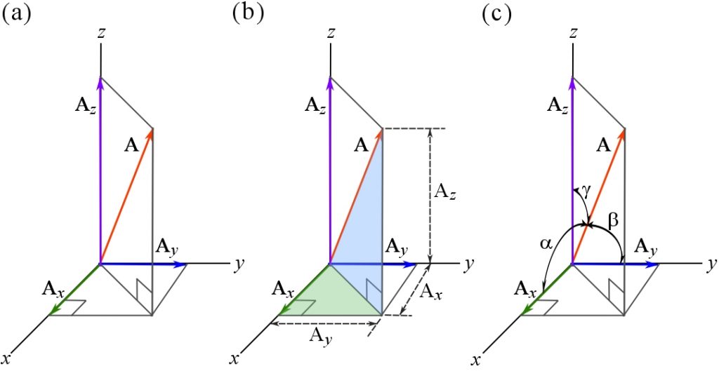
Figure 19. Components of a 3D vector in the 3D Cartesian coordinate system.
by its Cartesian components  . Dividing this equation by the magnitude of gives
  which is written as
  . Noting that
  is a unit vector, and taking the magnitude of the right hand side of the equation, we find the following relationship:

This means knowing two of the angles, the third one is readily obtainable.
Spatial vector operations using CVN (three dimensions)
Once the vectors to be summed are resolved into their components, the same steps as in the planar case should be followed but with including components in the direction. This means:
(4) ![\[\bold R=(\sum F_x)\bold i + (\sum F_y)\bold j + (\sum F_z)\bold kj \]](https://engcourses-uofa.ca/wp-content/ql-cache/quicklatex.com-2a44106eddede009497a2a37f599dbf9_l3.png "Rendered by QuickLaTeX.com")
in which , , and  represent the algebraic sums of the scalar components along the , and axes respectively.
Position vector
Naturally, we can have a perception of a geometric point in space. A point in the space (3D or 2D) can be imagined as an infinitely small dot. The space containing all the geometric points is called the geometric space. In a geometric space, geometric objects (or shapes) are born out of points. For examples, lines, circles, polylines, polygons, surfaces, cubes, etc. We simply refer to the geometric space as the space. The location of a point is the space can be quantitatively determined relative to other points. Thereby, all points can be located relative to one marked point. This point is called the origin of the space and denoted by . Generally, we form a Cartesian coordinate system in the space and define the origin of the space to be at the intersection of the three (or two) axes of the coordinate system. Therefore, any point in the space is identified by a coordinate triple  in the 3D space, or
  in the 2D space. Obviously, the coordinate of the origin is
  . This approach was introduced by the French mathematician and philosopher René Descartes.
Another approach to locate (identify) a point in the space is by using a vector. Once a point in the space is marked as the origin, a vector (arrow) can be readily drawn (imagined) from the origin of the space, , to any point, , in the space. This vector is called the position vector. The position vector is generally denoted by  . To indicate a particular point located by a position vector, the notation
  or
or  is used. The former notation explicitly express the sense of the direction from the origin to the point , while the latter notation implicitly conveys the sense of the direction. A position vector simply points at a point in the space; is tail is at the origin of the space and its head is at any point to be located (Figure 20a). Constructing a Cartesian coordinate system a the origin as well, the position vector is resolved by the CVN as:
![\[\bold r = x\bold i + y\bold j + z\bold k\]](https://engcourses-uofa.ca/wp-content/ql-cache/quicklatex.com-b49b77a979b7e9188068c68099a83c47_l3.png "Rendered by QuickLaTeX.com")
where are the coordinates of the point located by the position vector. Figure 20a shows a position vector in a Cartesian coordinate system locating the points of a space. Choosing a point as the origin of the space is arbitrary; however, a wise choice depending on the problem can simplify the equations. Figure 20b shows a point in a space located by two different coordinate systems and position vectors. Note that the point is the same point but looked at from two different outlooks; therefore it has different coordinates and position vectors in different coordinate systems.
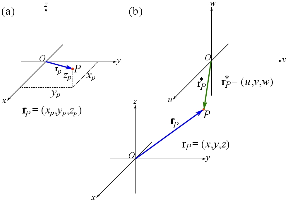
Figure 20. Position vector and coordinate systems.
 has the dimension and units of length, and it measures the distance between two points.
Remark: unit of a position vector or its length has to be specified and written in the calculations. For example you can write  where
where  are the scalar components with the dimension and unit of length, or for example
  .
.
Remark: the unit vector  has no dimension. The unit vectors (
 ) of the coordinate system have no dimension as well.
Using the coordinate direction angles , , and (measured from the positive , , and axes respectively), the following equations hold for a position vector in the Cartesian coordinate system:
(5) ![\[ \begin{split} \bold r &= x\bold i + y\bold j + z\bold k\quad\quad r=\vert\bold r\vert=\sqrt{x^2+y^2+z^2}\\ x&=r\cos \alpha\quad y=r\cos \beta\quad z=r\cos \gamma\quad \text{for } 0^\circ \le \alpha, \beta,\gamma \le 180^\circ\\ \bold r&=r \hat{\bold r}\ \text{such that }\hat{\bold r}=(\cos\alpha)\bold i +(\cos\beta)\bold j+(\cos\gamma)\bold k \end{split}\]](https://engcourses-uofa.ca/wp-content/ql-cache/quicklatex.com-378b3b714eab06b8c5693ae00f8cd554_l3.png "Rendered by QuickLaTeX.com")
Any vector in the geometric space is a type of a position vector because it connects two points whether or not either marked as the origin. If a (geometric) vector connects two points, say and  , in the space such than non of the points are designated as the origin, the vector is denoted by
  and called a displacement vector. The displacement vector in fact expresses the displacement of the position vector from point to point . To understand this concept, imagine two points and respectively located by the position vectors
  and
and  in the space already having a defined origin and a Cartesian coordinate system (Figure 21). The vector (arrow) from the point to the point is the displacement vector . By the rules of vector addition, we can write:
(6) ![\[\bold r_A+\bold r_{AB}=\bold r_B \quad\text{or}\quad \bold r_B-\bold r_A=\bold r_{AB}\]](https://engcourses-uofa.ca/wp-content/ql-cache/quicklatex.com-e3623fd188612c2dd749bb8f42103702_l3.png "Rendered by QuickLaTeX.com")
By using the CVN:
(7) ![\[\bold r_{AB}= (x_B-x_A)\bold i+(y_B-y_A)\bold j+(z_B-z_A)\bold k\]](https://engcourses-uofa.ca/wp-content/ql-cache/quicklatex.com-6b132f7d7cebee2b2d095b83e814caa0_l3.png "Rendered by QuickLaTeX.com")
Interpreting the above equations geometrically, we understand that if an object is displaced along the vector , its position is changed from the point , located by , to the point located by  . The quantity
  is the length of displacement.

Figure 21. Position and displacement vectors.
and in the space. This can be easily achieved through normalizing by writing  . It should be noted that another possibility for setting a direction is normalizing
  which is in the opposite direction of .
Dot product
The dot product, also called the scalar product, is an operation that takes two vectors and returns a scalar. The dot product of vectors and , denoted as  and read “ dot ” is defined as:
(8) ![\[\bold A\cdot\bold B=AB\cos \theta \]](https://engcourses-uofa.ca/wp-content/ql-cache/quicklatex.com-22c2def816d90defe8a272bb9b50a7ab_l3.png "Rendered by QuickLaTeX.com")
where  ,
,  , and
, and  is the angle between the two vectors (Figure 22)
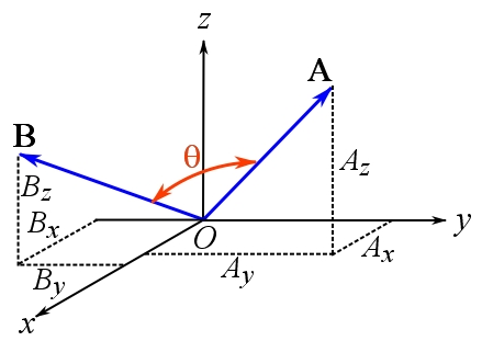
Figure 22. Configuration of two vectors for the dot product.
- Commutativity:

- Associativity (scalar multiplication):

- Distributivity:

The proofs of the first two properties are by direct using the dot product definition (Eq. 8). The proof for the third property is by expanding the right hand side of the equation using the CVN notation and factoring the scalar components of . Dot product using the CVN is explained below.
Other properties of the dot product
- Dot product of a vector by itself gives its squared magnitude:
 .
. - Dot product of two perpendicular vectors is zero:
 .
. - If
 then
then  .
. - If
 then
then  .
. - Dot product by the zero vector is zero:
 .
.
These properties are easily proved by using Eq. 8.
Formulation of the dot product using CVN
Let and be two vectors with their scalar components  and
and  . Using the CVN, we can write:
![\[ \begin{split} \bold A\cdot \bold B&=(A_x\bold i +A_y\bold j+A_z\bold k )\cdot(B_x\bold i +B_y\bold j+B_z\bold k)\\ &\text{by the distributivity property}\\ &=A_xB_x(\bold i\cdot \bold i)+A_xBy(\bold i\cdot \bold j)+A_xB_z(\bold i\cdot \bold k)\\ &+A_yB_x(\bold j\cdot \bold i)+A_yBy(\bold j\cdot \bold j)+A_yB_z(\bold j\cdot \bold k)\\ &+A_zB_x(\bold k\cdot \bold i)+A_zBy(\bold k\cdot \bold j)+A_zB_z(\bold k\cdot \bold k) \end{split}\]](https://engcourses-uofa.ca/wp-content/ql-cache/quicklatex.com-ee7c7f6bd9a6e109a536ea2c405432bc_l3.png "Rendered by QuickLaTeX.com")
The dot product of the unit vectors, by the dot product properties, are:
![\[ \begin{split} \bold i \cdot \bold i&=\bold j \cdot \bold j=\bold k \cdot \bold k=1\\ \bold i \cdot \bold j&=\bold j \cdot \bold i=\bold i \cdot \bold k=\bold k \cdot \bold i=\bold j \cdot \bold k=\bold k \cdot \bold j=0 \end{split}\]](https://engcourses-uofa.ca/wp-content/ql-cache/quicklatex.com-237f2edc7c2d4616730306e6e168a050_l3.png "Rendered by QuickLaTeX.com")
Therefore,
(9) ![\[\bold A\cdot \bold B=A_xB_x+A_yB_y+A_zB_z\]](https://engcourses-uofa.ca/wp-content/ql-cache/quicklatex.com-2487d5202d87b8c4eb75ccca3104cc6e_l3.png "Rendered by QuickLaTeX.com")
This result expresses that the dot product of two vectors written in their CVN is obtained by multiplying their corresponding scalar components and summing over these product algebraically. Equation 9 indicates that calculating the dot product (Eq. 8) does not need the magnitudes of two vectors and the angle between them, if the vectors are resolved in the Cartesian system.
Application of the dot product: finding the angle between two vectors
Dot product can be used to find the angle formed between two vectors or two intersecting line. This property facilitate the calculations particularly when solving problems in three dimensions. The angle between two vectors is obtained by solving Eq. 8. for the angle term:
(10) ![\[\theta=\cos^{-1}(\frac{\bold A\cdot\bold B}{AB})\quad 0^\circ\le \theta\le 180^\circ \]](https://engcourses-uofa.ca/wp-content/ql-cache/quicklatex.com-693b07b2b6aba357e17f714aa1cfe86b_l3.png "Rendered by QuickLaTeX.com")
in which  is found from Eq. 9.
The above equation can be manipulated as:
![\[\theta=\cos^{-1}(\frac{\bold A}{A}\cdot\frac{\bold B}{B})=\cos^{-1}(\bold u_A\cdot\bold u_B)\quad 0^\circ\le \theta\le 180^\circ\]](https://engcourses-uofa.ca/wp-content/ql-cache/quicklatex.com-15cc5fa2e9cb80b895b79285450ba5f1_l3.png "Rendered by QuickLaTeX.com")
in which  and
and  are the unit vectors of and respectively. This result naturally states that the angle between two vectors only depends on their directions and not on their magnitudes.
Application of the dot product: orthogonal projection of a vector
In many problems, we need to resolve a vector on a particular line or lines in the space. To be more precise, the component of a vector along a particular direction or axis is to be found. Decomposing a vector onto the Cartesian axes is already demonstrated. In this section, we explain decomposing a vector on general lines or axes in space using the dot product. Using the dot product makes the calculation easier specially in three dimensions.
Consider a non zero vector in the three dimensional space and a line  intersecting the tail of the vector at a point (Figure 23a). This line accompanies the direction along which we want to decompose the vector. The positive direction of the line is determined by a unit vector say . As previously mentioned, a line along with a colinear vector (determining the positive direction) is called an axis. It is intended to resolve into two components as (Figure 23b):
(11) ![\[ \bold A =\bold A_a + \bold A_{\perp} \]](https://engcourses-uofa.ca/wp-content/ql-cache/quicklatex.com-2cfcdbd6b8a3b22c40e900e31745b936_l3.png "Rendered by QuickLaTeX.com")
where  is the component of parallel to (colinear with) the line and, indeed, the unit vector , and
  is the component of perpendicular to the line and, of course, the unit vector . The symbol
  denotes perpendicularity.

Figure 23. Orthogonal projection.
is called the parallel component of . Also, is referred to as the orthogonal projection (or projection) of onto the line or along the direction of . To obtain , it suffices to note that the vectors , and form a right-angle triangle (Figure 23b). Therefore by the Pythagorean’s theorem:
(12) ![\[ \begin{split} A_a=A\cos \theta&=\bold A\cdot\bold u_a \\ \bold A_a&=A_a\bold u_a\\ \vert\bold A_a \vert&=\mid A_a\mid \end{split}\]](https://engcourses-uofa.ca/wp-content/ql-cache/quicklatex.com-a61b6c08d2dee74d716deae7c28a2c1e_l3.png "Rendered by QuickLaTeX.com")
It should be noted that  is the scalar component of resolved along the direction of . Using the dot product
  to calculate may result in a negative scalar if the angle between
  and are larger than
  . In such a case, the direction of is in the opposite direction of .
The perpendicular component of can be then obtain by writing:
![\[ \bold A_{\perp}=\bold A-\bold A_a \]](https://engcourses-uofa.ca/wp-content/ql-cache/quicklatex.com-72e7add1545fe803103bf68ce60e9cf7_l3.png "Rendered by QuickLaTeX.com")
The magnitude of the perpendicular component can be calculated either by  or
or  .
.
In practice,  and can be readily used if
  in known, otherwise
  ,
,  , and can be utilized if the components of the vectors in CVN are known.
As a special case, orthogonal projection is used to find the scalar components of a vector in a Cartesian frame. This is done by writing:
(13) ![\[ \begin{split} A_x&=\bold A\cdot \bold i\\ A_y&=\bold A\cdot \bold j\\ A_z&=\bold A\cdot \bold k \end{split}\]](https://engcourses-uofa.ca/wp-content/ql-cache/quicklatex.com-42598afd087d6115d59a276db97e7317_l3.png "Rendered by QuickLaTeX.com")
Cross product
The cross product of two vectors is an operation that takes two vectors and and returns a vector . This operation is denoted by  and is read “C equals A cross B”. The resultant vector has a magnitude,
  ,and a direction denoted by
  .
.
For  The magnitude of is defined as:
(14) ![\[C=AB\sin\theta\quad\quad 0^\circ\le \theta \le 180^\circ\]](https://engcourses-uofa.ca/wp-content/ql-cache/quicklatex.com-6ad0e467d9f922062441b4eda32d3881_l3.png "Rendered by QuickLaTeX.com")
in which is the angle between the two vectors.
The definition of the magnitude of the cross product implies that,  if two non-zero vectors are colinear.
By definition, is perpendicular to both and which are not colinear and it is direction is specified by the right-hand rule. In other words, is perpendicular to the plane containing the non-colinear vectors and such that is in the direction of the thumb following the right-hand rule (Figure 24).
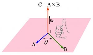
Figure 24. Cross product.
Properties of Cross product
- Anti-commutativity:

- Associativity: for a scalar
 ,
, 
- Distributivity:

Cross product in CVN
In a Cartesian frame the following relationships are readily obtained for the mutually perpendicular unit vectors , and :
![\[ \begin{matrix} \bold i\times \bold i=\bold 0 &\bold i\times \bold j=\bold k & \bold i\times \bold k=-\bold j \\ \bold j\times \bold i=-\bold k & \bold j\times \bold j=\bold 0 & \bold j\times \bold k=\bold i \\ \bold k\times \bold i=\bold j & \bold k\times \bold j=-\bold i & \bold k\times \bold k=\bold 0 \\ \end{matrix} \]](https://engcourses-uofa.ca/wp-content/ql-cache/quicklatex.com-5957262068ec49c412761182cc347572_l3.png "Rendered by QuickLaTeX.com")
Based on the above results and the properties of the cross product, the cross product of two vectors in their CVN is:
![\[ \begin{split} \bold A&=A_x\bold i + A_y\bold j+A_z\bold k\quad , \quad \bold B=B_x\bold i+B_y\bold j+B_z\bold k\\ \bold A\times \bold B&=(A_xB_x)\bold i\times \bold i +(A_xB_y)\bold i\times \bold j +(A_xB_z)\bold i\times \bold k\\ &+(A_yB_x)\bold j\times \bold i +(A_yB_y)\bold j\times \bold j +(A_yB_z)\bold j\times \bold k \\ &+(A_zB_x)\bold k\times \bold i +(A_zB_y)\bold k\times \bold j +(A_zB_z)\bold k\times \bold k \end{split}\]](https://engcourses-uofa.ca/wp-content/ql-cache/quicklatex.com-b289cdf6a59bd07c0bf55e299f6aac27_l3.png "Rendered by QuickLaTeX.com")
leading to:
![\[ \bold A\times\bold B=(A_yB_z-A_zB_y)\bold i+(A_zB_x-A_xB_z)\bold j+(A_xB_y-A_yB_x)\bold k \]](https://engcourses-uofa.ca/wp-content/ql-cache/quicklatex.com-e65afe746ec8995f33a8a646717f0771_l3.png "Rendered by QuickLaTeX.com")
This result need not to me memorize and can be obtained by calculating the following determinant symbolically:
(15) ![\[ \bold A\times\bold B = \begin{vmatrix} \bold i & \bold j & \bold k \\ A_x & A_y & A_z \\ B_x & B_y & B_z \\ \end{vmatrix}\]](https://engcourses-uofa.ca/wp-content/ql-cache/quicklatex.com-77d6966ef6d0f5d0200f157a3177907a_l3.png "Rendered by QuickLaTeX.com")