Engineering at Alberta Courses » Point Collocation Method

Approximate Methods: Point Collocation Method

The statement of the equilibrium equations applied to a set $D\subset\mathbb{R}^3$ is as follows. Assuming that at equilibrium $\sigma:D\rightarrow\mathbb{M}^3$ is the symmetric Cauchy stress distribution on $D$ and that $u:D\rightarrow\mathbb{R}^3$ is the displacement vector distribution and knowing the relationship $\sigma=\sigma(u)$ , then the equilibrium equation seeks to find $u\in U$ such that the associated $\sigma$ satisfies the equation:

$\mathrm{div}\sigma+\rho b= 0$

where $b:D\rightarrow\mathbb{R}^3$ is the body forces vector distribution on $D$ , $\rho$ is the mass density, and $U$ is the space of all possible displacement functions applied to $D$ , i.e., $U=\{a:D\rightarrow\mathbb{R}^3| a\mbox{ is kinematically admissible}\}$ . The term “Kinematically admissible” in $U$ indicates that the space of possible solutions must satisfy the boundary conditions imposed on $\partial D_u$ (as stated below) and any differentiability constraints.

The boundary conditions for the equations of equilibrium are usually given on two parts of the boundary of $D$ denoted $\partial D$ . On the first part, $\partial D_n$ , the external traction vectors $t_n$ are known so we have the boundary conditions for $\sigma$ since $\sigma^Tn=t_n$ ( $n$ is the normal vector to the boundary). On the second part, $\partial D_u$ , the displacement is given.

The point collocation method seeks an approximate solution to the above problem by assuming that the solution $u$ has a particular form with a finite number of unknowns, i.e., by looking for $u$ in a subset $U_{fd}\subset U$ that is finite dimensional but still able to approximate functions in $U$ . The finite number of unknowns can be found by satisfying the differential equation of equilibrium at a number of chosen points equal to the number of unknowns.

Example

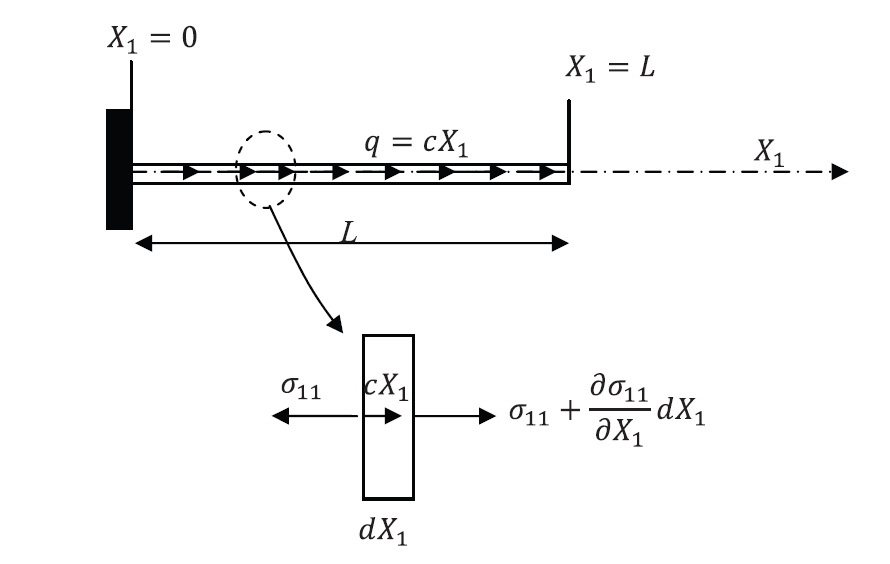
Using a polynomial function of the third degree, find the displacement function of the shown bar by satisfying the essential boundary conditions, the differential equation of equilibrium at $X_1=\frac{L}{2}$ and at $X_1=L$ ., and the nonessential boundary condition at $X_1= L$ . Assume that the bar is linear elastic with Young’s modulus $E$ and cross-sectional area $A$ and that the small strain tensor is the appropriate measure of strain. Ignore the effect of Poisson’s ratio.
PL1

Solution

Exact Solution

The exact solution can be obtained by directly solving the differential equation of equilibrium utilizing $\sigma_{11}=E\frac{\mathrm{d}u_1}{\mathrm{d}X_1}$ :

$\frac{\mathrm{d}^2u_1}{\mathrm{d}X_1^2}=-\frac{cX_1}{EA}$

with the boundary conditions: $@X_1=0:u_1=0$ and $X_1=L:\frac{\mathrm{d}u_1}{\mathrm{d}X_1}=0$ .
Therefore:

$u_1=\frac{cL^2}{2EA}X_1-\frac{c}{6EA}X_1^3$

View Mathematica Code

DSolve[{u''[X1] == -c*X1/EA, u'[L] == 0, u[0] == 0}, u[X1], X1]

Approximate Solution

A polynomial of the third degree approximate solution has the form:

$u_{approx}=a_0+a_1X_1+a_2X_1^2+a_3X_1^3$

with

$\begin{split} \frac{\mathrm{d}u_{approx}}{\mathrm{d}X_1}&=a_1+2a_2X_1+3a_3X_1^2\\ \frac{\mathrm{d}^2u_{approx}}{\mathrm{d}X_1^2}&=2a_2+6a_3X_1 \end{split}$

The following four equations will be utilized to find the four unknowns:

$\begin{split} @X_1=0&:u_{approx}=0\\ @X_1=L&:\frac{\mathrm{d}u_{approx}}{\mathrm{d}X_1}=0\\ @X_1=\frac{L}{2}&:\frac{\mathrm{d}^2u_{approx}}{\mathrm{d}X_1^2}\bigg|_{X_1=\frac{L}{2}}=-\frac{cX_1}{EA}\bigg|_{X_1=\frac{L}{2}}\\ @X_1=L&:\frac{\mathrm{d}^2u_{approx}}{\mathrm{d}X_1^2}\bigg|_{X_1=L}=-\frac{cX_1}{EA}\bigg|_{X_1=L} \end{split}$

The approximate solution that satisfies the above four unknowns has the form:

$u_{approx}=\frac{cL^2}{2EA}X_1-\frac{c}{6EA}X_1^3$

Notice that since the exact solution is contained in the space of approximate functions which were chosen to satisfy both the essential and nonessential boundary conditions, the solution obtained is indeed the exact solution!
View Mathematica Code

u = a0 + a1*x1 + a2*x1^2 + a3*x1^3;
ux = D[u, x1]
uxx = D[ux, x1]
Eq1 = (uxx + c*x1/EA) /. x1 -> L/2;
Eq2 = (uxx + c*x1/EA) /. x1 -> L;
Eq3 = (ux) /. x1 -> L;
Eq4 = u /. x1 -> 0;
s = Solve[{Eq1 == 0, Eq2 == 0, Eq3 == 0, Eq4 == 0}, {a1, a2, a3, a0}]
u /. s[[1]]

Open Educational Resources

Approximate Methods: Point Collocation Method

Example

Solution

Exact Solution

Approximate Solution

Leave a Reply Cancel reply